In our quest to understand the mathematical architecture of machine learning, we hopped on to a new destination where the objective is to uncover the precise mechanics of how algorithms acquire knowledge. We will navigate through the framework of Calculus - mainly focussing on Differential Calculus, from foundational single variable functions to complex multi-variable systems, grasping how they actually capture the dynamics of the underlying system and bring insights facilitating the learning process. In this comprehensive six-part series we will start from the core fundamentals and gradually ascend to more complicated concepts that power contemporary Artificial Intelligence AI.
What is a Machine?
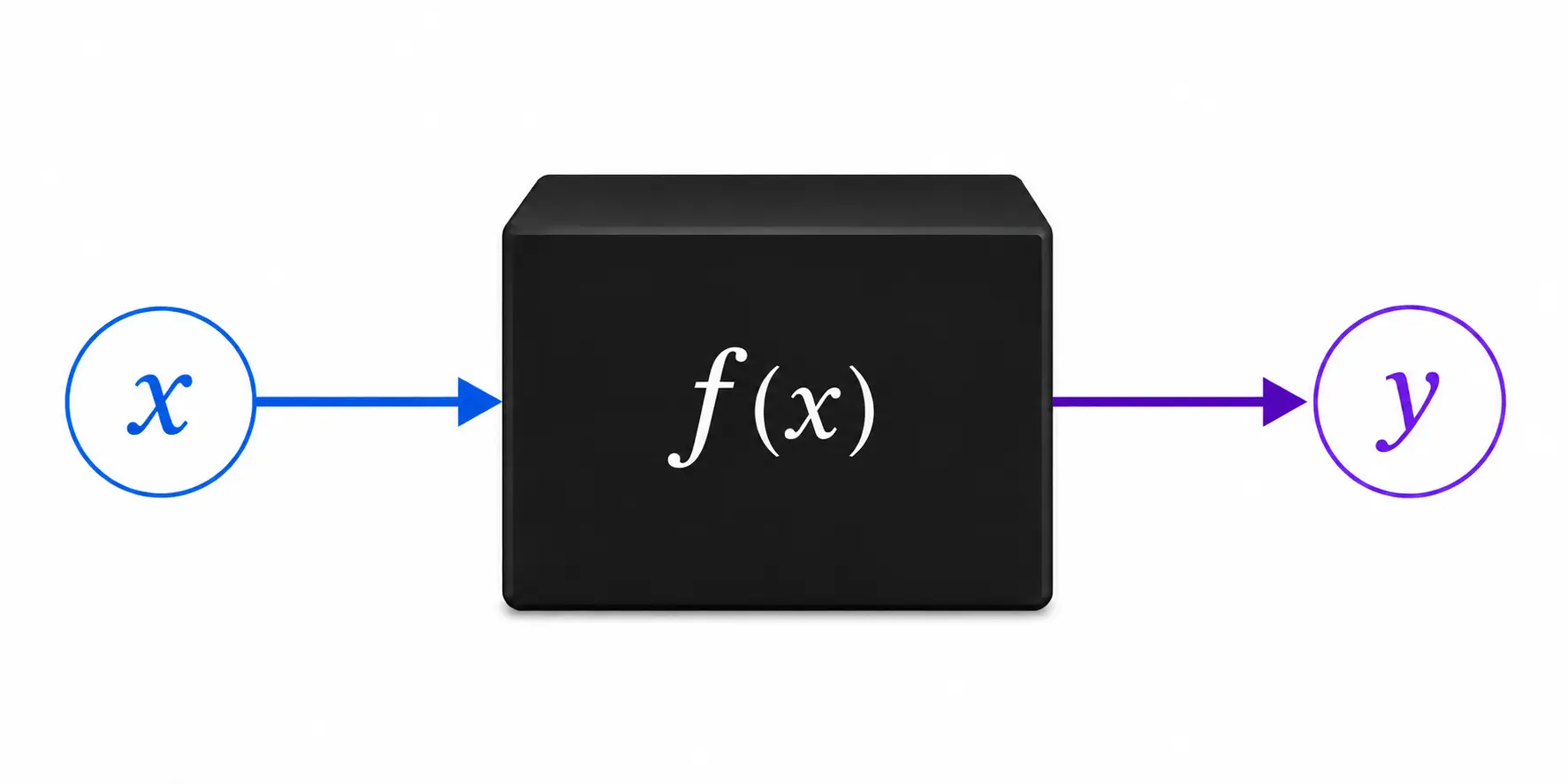
Traditionally when we think of a machine, we only imagine a physical device that takes some input and produces some tangible finished products. The same definition holds in the fields of AI too that an output \(y\) is produced from input \(x\) by a machine defined as \(f(x)\).
The Core of Learning
What is to be learnt? The simple answer is - the machine needs to know the process to translate \(x\) to \(y\). The idea is to teach the machine how to draw insights from the input provided and identify hidden patterns in the input which evolves into its learning and enables it to make accurate predictions.
The Framework of Machine Learning
The only difference between “machine” in machine learning ML and traditional devices is that the output is digital for the former and hence intangible. There is no direct recipe in ML; rather ML algorithms tell the machine about the learning Objective and how to recognize patterns to complete the effective learning to reach that objective and acquire sufficient knowledge about the input data so that accurate predictions can be generated on new observations. Once we dive deep into the fields of AI/ML we can easily comprehend that the machine in ML is an illusion; it is the algorithm only that adjusts its parameters to learn.
The Optimization Engine
Learning in AI or ML is an iterative process. The iteration begins when the algorithm does not have any understanding of the patterns in the input data and ends when it sufficiently acquired knowledge about the input. Now the obvious question is how to quantify “No” or “Sufficient”! The answer lies with the role played by another entity - Loss Function. Loss function has a specific mathematical formulation and it helps algorithms to measure the gap in its understanding termed as “Error” which is defined as the difference between actual output and predicted output. So when the error is large, we can say algorithms haven’t learnt anything and when error is low, we can safely assume that it has learnt enough and the learning process has converged.
Let’s assume the loss function is defined as the absolute deviation between actuals and prediction then here is a simple Python implementation to implement this.
def loss_function(actual, prediction):
    loss = round(abs(actual - prediction), 2)
    print("Loss is: " + str(loss))
    return loss

loss_pred1 = loss_function(5, 5.1)
loss_pred2 = loss_function(5, 5.2)

if loss_pred1 > loss_pred2:
    print("Prediction 2 is better!")
else:
    print("Prediction 1 is better!")
It generates the loss for predictions 5.1 and 5.2 against the actual value of 5.
Loss is: 0.1
Loss is: 0.2
Prediction 1 is better!
This is a toy example showing how loss function drives the decision making of which prediction is better and helps the algorithm to fine tune its learning.
Following the Slopes
The above example is a one-step approach and the real crux lies when we have to follow multiple iterations to understand what is better. In the iterative process if we have two possibilities at each iteration, then the prediction that reduces the maximum gap with actual value should be chosen. We start with the maximum gap possible because of no learning initially, begin to “minimize” the gap over the iterations as we continue to choose the best one at each step and finally stop when loss function indicates that no further significant improvement in learning is possible.
Let’s try to build an analogy with hill climbing or descending from a hill to better link concepts of differential calculus with machine learning. At the bottom of a hill, there is a plain with slope zero and we are in our car. Our objective is to reach the hill top. As we start driving, how do we know if we have taken the right path and ascending? Similarly, when we intend to descend from the hill top how do we know if we are actually descending? These questions can be answered if we are able to calculate the steepness of the road at the current location and follow the direction of steepest ascent (to reach uphill) and steepest descent (to reach downhill). Do you know what is meant by steepness in differential calculus - the Slope calculated using the Derivative! The slope is actually the optimization engine that powers the decision of whether we are on the right track and whether we have reached the summit or the foothills is controlled by the loss function.