
In the first blog of this series we tried to connect the dot between Machine Learning ML and Calculus. We ended up with concepts such as learning objective, cost function as a measure of determining whether we have reached the objective and iteratively we calculate the loss as a metric of determining how far we are from reaching our objective basis the cost function and we try to reduce the gap as much as possible. We will see later that the same concepts apply to Deep Learning DL as well.
What is a Derivative?
The bird’s eye view of the purpose of ML and DL (together, AI) is to find a mapping that best describes the relationship between output with respect to input.
$$ y = f(x) $$
But how will the output \(y\) behave when there is a small change in the input \(x\). Question is why is it important to know the change in \(y\) with respect to \(x\). Let’s think about the marks in an exam; if a student studies 5 hours a day then s/he gets 50 out of 100. If the same student studies 6 hours a day and gets 55, so how much marks will s/he get if s/he continues to study for 8 hours? To answer this question, we need to know the rate at which additional marks are scored based on the change in study hours.
To measure the rate we can capture the value of \(y\) at value \(x\) and \(x + \Delta x\) where \(\Delta x\) is the change in the value of \(x\). Then the rate of change of \(y\) becomes,
$$ \frac{\Delta y}{\Delta x} = \frac{f(x + \Delta x) - f(x)}{\Delta x} $$
The rate can thus be expressed in terms of the slope of the secant line passing through two points - \({P: (x, f(x)), Q: (x + \Delta x, f(x + \Delta x))}\) on the graph of \(y = f(x)\).
When \(\Delta x\) is small, the limiting value of the rate forms the instantaneous change of \(y\) with respect to \(x\) and the secant line becomes the tangent line at \(P\) which is nothing but the derivative of \(y\) with respect to \(x\).
$$ \lim_{\Delta x \to 0} \frac{\Delta y}{\Delta x} = \lim_{\Delta x \to 0} \frac{f(x+\Delta x) - f(x)}{\Delta x} = f’(x) = \frac{dy}{dx} $$
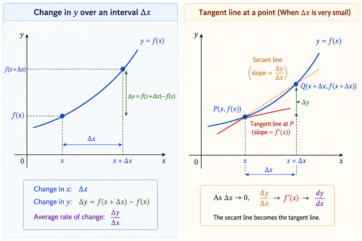
In AI, we need to find out this rate of change of output \(y\) with respect to input \(x\) to gauge the variation of output on the basis of changes in input which ultimately can be summarized as the learning process.
The derivative of the first derivative is called the Second/Double Derivative and has particular use cases e.g. speed and acceleration of a car. The second derivative has a special significance that will be discussed in the next blog.
$$ \text{Speed} = \text{first derivative} = \frac{\text{change in displacement}}{\text{change in time}} $$
$$ \text{Acceleration} = \text{second derivative} = \frac{\text{change in speed}}{\text{change in time}} $$
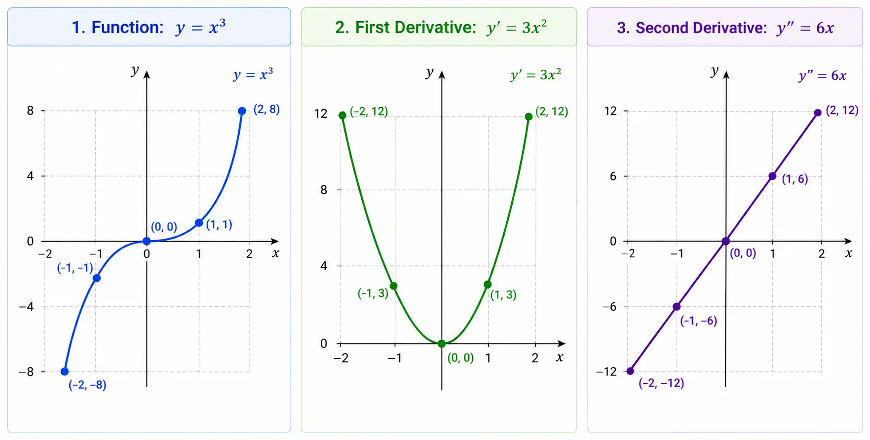
For a function \(y = x^3\), the first and second derivatives are plotted below respectively.
Intuition behind Chain Rule
Think about our previous example of obtaining marks in the exam where marks obtained \(M\) is dependent on hours of study \(S\) and bring another dimension to it. Let’s consider hours of study is also dependent on hours of sleep \(L\) and we want to find out the rate of change of \(M\) with unit change of \(L\). But \(M\) is not directly connected to \(L\).
Mathematically,
$$ M \to f(S) \quad \text{and} \quad S \to f(L) $$
So, the rate of change of \(M\) with unit change of \(L\) can be expressed in terms of the rate of change of \(M\) with unit change of \(S\) and the rate of change of \(S\) with unit change of \(L\). This is called the Chain Rule.
$$ \frac{dM}{dL} = \frac{dM}{dS} \cdot \frac{dS}{dL} $$
Scaling to Higher Dimensions
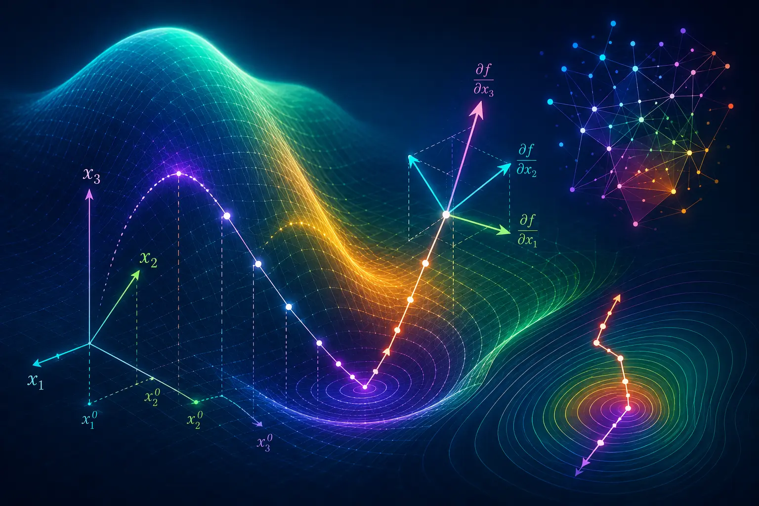
In reality, there are multiple factors that affect a particular outcome. For example, the resale value \(V\) of a house is dependent on its floor-area \(F\) and age \(A\). So, we enter into multivariate landscape where
$$ y = f(x_1, x_2, …, x_n) $$
$$ V = f(F, A) $$
In the multivariate scenario all the concepts of slope, first derivative and second derivative hold but with a different nomenclature.
Partial Derivative
When only one factor is changed keeping the other factor(s) constant, the derivative is called Partial Derivative. In our example, partial derivatives (represented with \(\partial\) sign) are
$$ \frac{\partial V}{\partial F} \quad \text{and} \quad \frac{\partial V}{\partial A} $$
They represent the rate of change of resale value with respect to floor-area and age respectively.
Gradient
If all the first order partial derivatives are stacked as a vector then they form Gradient.
$$ \nabla V = \left[ \frac{\partial V}{\partial F}, \frac{\partial V}{\partial A} \right]^T $$
Hessian
The second order partial derivatives are calculated to form the Hessian matrix. Hessian captures the curvature of the resale value.
$$ H = \begin{bmatrix} \dfrac{\partial^2 V}{\partial F^2} & \dfrac{\partial^2 V}{\partial F \partial A} \\ \dfrac{\partial^2 V}{\partial F \partial A} & \dfrac{\partial^2 V}{\partial A^2} \end{bmatrix} $$
Consider, the resale value \(V\) has the form below -
$$ V = F^3 \cdot A^3 $$
Then,
$$ \text{Gradient} \quad \nabla V = \begin{bmatrix} 3F^2A^3 & 3F^3A^2 \end{bmatrix}^T $$
$$ \text{Hessian} \quad H = \begin{bmatrix} 6FA^3 & 9F^2A^2 \\ 9F^2A^2 & 6F^3A \end{bmatrix} $$
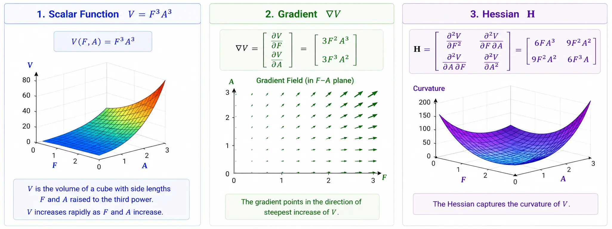
Here is a simple Python implementation of symbolic calculation of Gradient and Hessian of the above example.
import sympy as sp

def calculate_gradient_and_hessian():
    # 1. Define the symbolic variables
    F, A = sp.symbols('F A', real=True)

    # 2. Define the objective function V = F^3 * A^3
    V = (F**3) * (A**3)
    print("--- Original Function ---")
    sp.pprint(sp.Eq(sp.Symbol('V'), V))
    print("\n")

    # 3. Calculate the Gradient Vector
    dV_dF = sp.diff(V, F)
    dV_dA = sp.diff(V, A)
    gradient = sp.Matrix([dV_dF, dV_dA])
    print("--- Gradient Vector ---")
    sp.pprint(gradient)
    print("\n")

    # 4. Calculate the Hessian Matrix
    d2V_dF2 = sp.diff(V, F, 2)
    d2V_dA2 = sp.diff(V, A, 2)
    d2V_dFdA = sp.diff(sp.diff(V, F), A)  # Mixed partial derivative
    hessian = sp.Matrix([[d2V_dF2, d2V_dFdA],
                          [d2V_dFdA, d2V_dA2]])
    print("--- Hessian Matrix ---")
    sp.pprint(hessian)
    print("\n")

if __name__ == "__main__":
    calculate_gradient_and_hessian()