For an AI algorithm the learning process is an iterative way of maximizing its understanding of the input and minimizing the gap between algorithm’s output and actual values. It appears to be riding on top of loss function and taking a gradual descent in each iteration. But how does the process identify what is the direction of descent? How does the algorithm determine if it is actually learning? The answer lies in the interpretation of derivative and its multi-variable counterpart - gradient that provides the direction of descent and enables a framework for the algorithm to learn in a repetitive manner.
The Gradual Descent
In the famous descending from a hill example in the first blog, we discussed the slope of the hill measured by the derivative provides the steepness across different directions. If we follow the direction of maximum steepness and navigate to the downhill we can be sure that we will gradually descend to the plain. Gradient Descent is the mathematical framework that defines this.
In any machine learning use case, the training process involves learning the parameters through which the model can map the output from input. In each iteration of the process, once the model parameters are learnt, predictions are generated on the seen observations and the gap between actuals and predictions (error) is captured. The training objective is to sufficiently learn those model parameters in such a way that the error is minimal once the learning is complete.
Let’s consider the gradient descent for linear regression defined as \(y = wx + b\). The objective of the learning process is to find out the best \(w\) and \(b\).
The cost function is the sum of mean squared error between actual and prediction of \(m\) observations.
$$ Loss\ J(w,b) = \frac{1}{m}\sum_{i=1}^{m} (y_{act_i} - y_{pred_i})^2 $$
$$ Loss\ J(w,b) = \frac{1}{m}\sum_{i=1}^{m} (y_{act_i} - (wx_i + b))^2 $$
Partial derivative of loss with respect to slope \(w\),
$$ \frac{\partial J}{\partial w} = -\frac{2}{m}\sum_{i=1}^{m} x_i (y_{act_i} - y_{pred_i}) $$
Partial derivative of loss with respect to intercept \(b\),
$$ \frac{\partial J}{\partial b} = -\frac{2}{m}\sum_{i=1}^{m} (y_{act_i} - y_{pred_i}) $$
Since we want to follow the direction of steepest descent to minimize the gap i.e. reach downhill we will update \(w\) and \(b\) as below.
$$ \begin{aligned} w_{new} &\leftarrow w_{old} - \eta \cdot \frac{\partial J}{\partial w} \\ b_{new} &\leftarrow b_{old} - \eta \cdot \frac{\partial J}{\partial b} \end{aligned} $$
This process continues until the stopping criteria is met which can be the number of iterations or minimum error tolerance.
Gradient descent in its true form operates over all observations of the input, if it works on each observations randomly then it is called as Stochastic Gradient Descent and when it performs the gradient descent on a random subset of observations, it is termed as Batch Gradient Descent.
In the update rule, one important parameter is \(\eta\) called the learning rate or step size that controls how much the values are nudged and acts as a multiplier of the gradient. If it is large then the learning is faster and when it is small, the learning is slower.
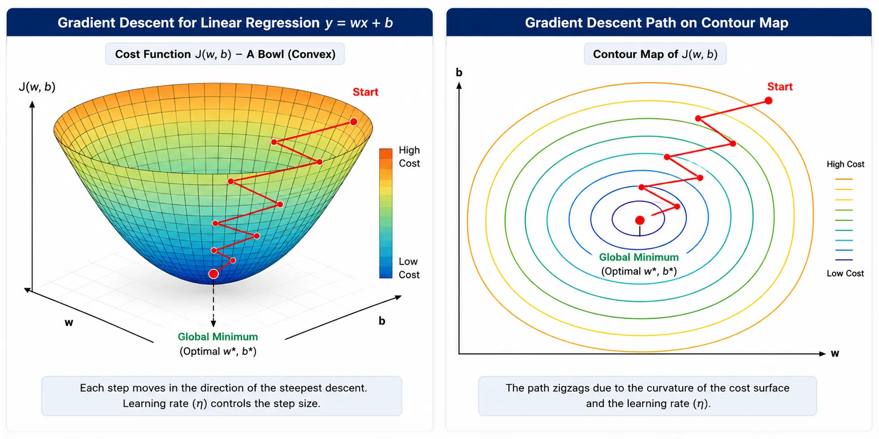
In the left hand side of the below image, we are seeing the 3D view of the cost function. Now at each step the algorithm reaches a new point along the curved edge of the 3D view. If we squash those curved lines containing those points into 2D we get semi-concentric circles with the global minimum at the centre. This view is called the Contour Map.
The Critical Points
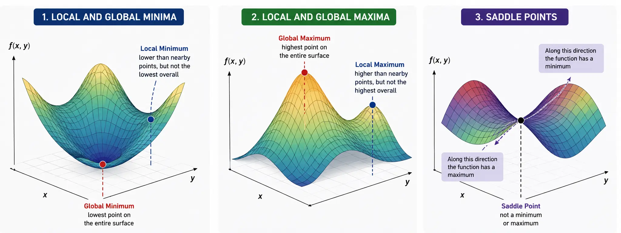
Critical points of a function represent specific locations where the slope is zero or undefined. It can be of three types - maxima, minima and saddle point but they have one thing in common - the derivative of the function at those points is zero under normal circumstances.
Minima
For any distribution (both single and multi-variable cases), there are few points where the value of the function is less compared to the value at other points in the close vicinity. These points are called Local Minima. The point where the function value is absolutely lowest is called Global Minima.
Maxima
Similarly, for any distribution (both single and multi-variable cases), there are few points where the value of the function is more compared to the value at other points in the close proximity. These points are called Local Maxima. The point where the function value is absolutely highest is called Global Maxima.
Saddle Points
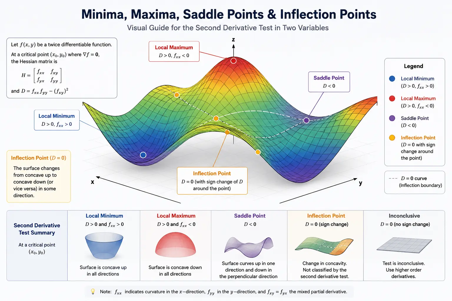
There can be few points for a distribution (both single and multi-variable cases) where the slope is zero in all directions; it can appear as maxima from one direction and minima from another direction. So the points which are neither maxima nor minima are termed as Saddle Points. A saddle point can become an Inflection Point if the concavity shifts from up to down and vice versa in any direction across that point.
The Second Derivative Test
Now the question comes to how we determine if a point on a function is maxima, minima or a saddle point. The process is called Second Derivative test and the approach is similar for single and multi variable scenarios and the core concept is zero slope at critical points. Double derivative test uses the curvature of the function to determine this.
Single-Variable Scenario
When there is single independent variable, the process is:
- Calculate derivative of the function.
- Set derivative = 0 and solve for that independent variable to get the critical point(s).
- Evaluate second derivative at each of the critical points and if a. If the second derivative at critical point > 0, the function is convex and the critical point is local minimum. b. If the second derivative at critical point < 0, the function is concave and the critical point is local maximum. c. If the second derivative at critical point = 0, the test is inconclusive and the critical point can be a maxima, minima or saddle point.
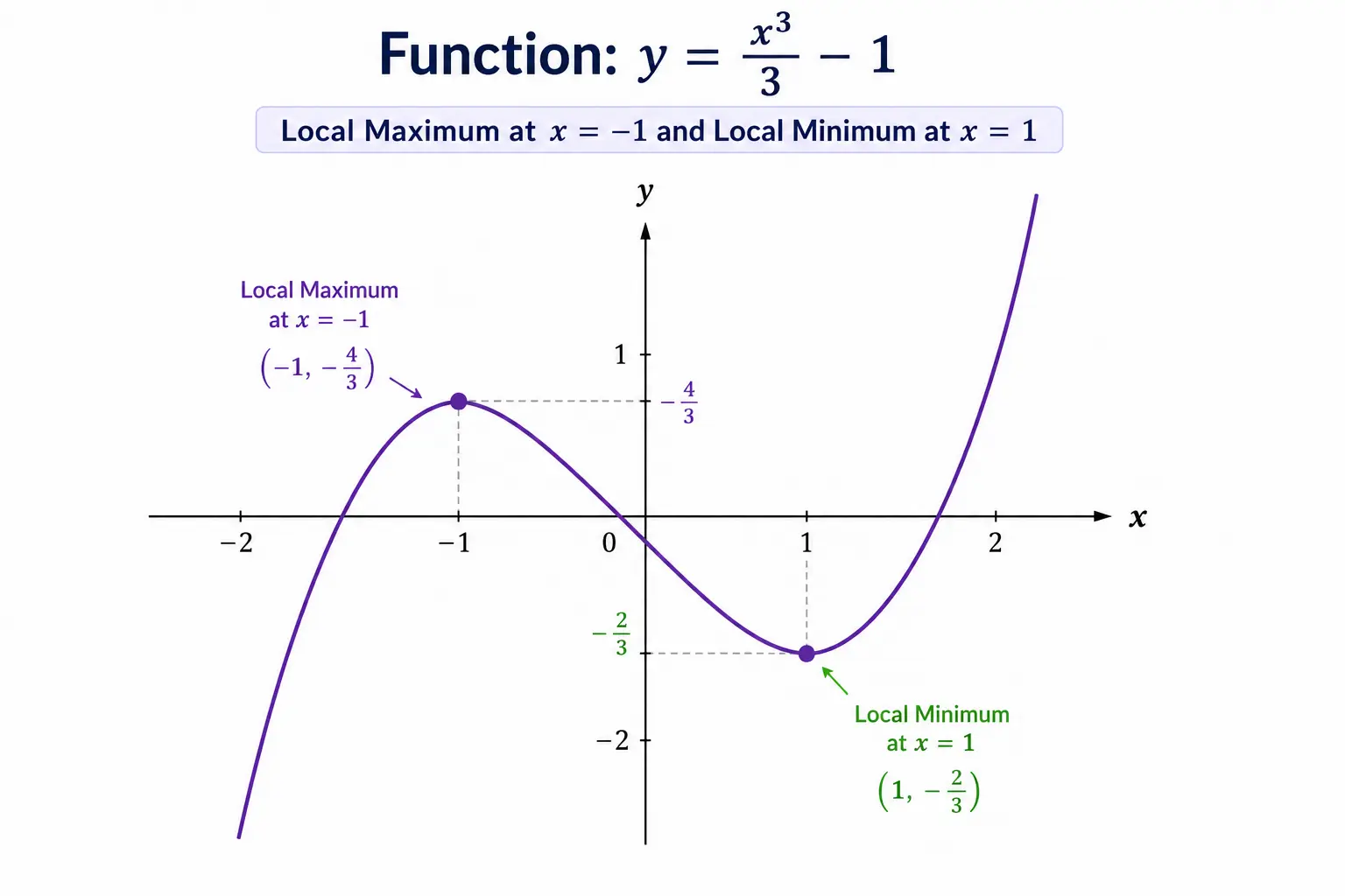
Let’s consider below function, its first and second derivatives as -
$$ y = \frac{x^3}{3} - x $$
$$ \frac{dy}{dx} = x^2 - 1 $$
If we solve the equation \(\frac{dy}{dx} = 0\) then \(x=+1\) and \(x=-1\) are the critical points.
Second derivative is -
$$ \frac{d^2y}{dx^2} = 2x $$
which results in \(+2\ (> 0)\) for \(x=+1\) and \(-2\ (< 0)\) for \(x=-1\). So, the critical point \(x=+1\) is a local minima and \(x=-1\) is a local maxima.
Multi-Variable Scenario
When there are multiple independent variables, the process is:
- Calculate gradient of the function.
- Set gradient = 0 and solve for the independent variables to get the critical point(s).
- Generate the hessian matrix of the function with the form below -
$$ H = \begin{bmatrix} f_{xx} & f_{xy} \\ f_{yx} & f_{yy} \end{bmatrix} $$
- Calculate the determinant \(D\) of the matrix as \(f_{xx} \cdot f_{yy} - f_{xy} \cdot f_{yx}\).
- If \(D > 0\), a. If \(f_{xx}\) at critical point > 0, the function is convex and the critical point is local minima. b. If \(f_{xx}\) at critical point < 0, the function is concave and the critical point is local maxima.
- If \(D < 0\), the critical point is the saddle point.
- If \(D = 0\), the test is inconclusive.
Let’s take the following function,
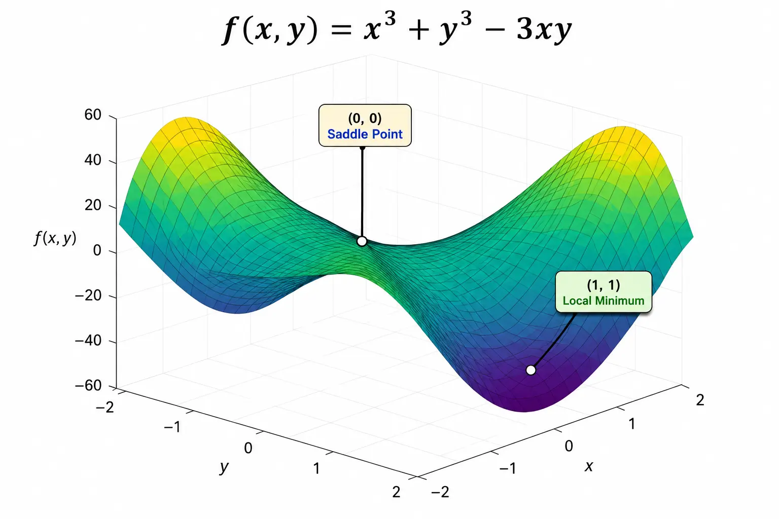
$$ f(x, y) = x^3 + y^3 - 3xy $$
Solving the gradient we get the critical points as -
$$ 3x^2 - 3y = 0 \Rightarrow y = x^2 $$
$$ 3y^2 - 3x = 0 \Rightarrow x = y^2 $$
From equations \(y = x^2\) and \(x = y^2\), the critical points are calculated as \((0, 0)\) and \((1, 1)\).
The hessian matrix is
$$ H = \begin{bmatrix} 6x & -3 \\ -3 & 6y \end{bmatrix} $$
Determinant \(D\) is \(36xy - 9\) and is \(-9\) and \(27\) respectively at \((0, 0)\) and \((1, 1)\). As per the logic mentioned above, point \((0, 0)\) is a saddle point because \(D < 0\); at point \((1, 1)\), \(D > 0\) and \(f_{xx} = 6x = 6 > 0\) signifying it as a local minima.
The following visual summarizes the concepts.
Lagrange Relaxation
We are able to establish the fact that gradient descent is an optimization process that iteratively reaches the local minima. In any optimization process there is an objective function that gets optimized with respect to a set of constraints.
We can think of a scenario where we want to reduce the transportation cost and have two options - one which costs INR 10000 and another which costs INR 12000. But we have a constraint that the cost should be within INR 8000. Under this constraint we cannot select any option. If we calculate the additional cost for each of these options then we will get INR 2000 and INR 4000. Now if we consider these additional costs (penalty) along with our original objective function then we form a relaxed version of the original optimization problem which is solvable. In this relaxed set up, option-1 will be selected because of having less penalty. This is called Lagrange Relaxation.
Mathematically,
$$ \text{Original problem,} \quad \text{Min } c^T X \text{ subject to } AX \le b $$
$$ \text{Relaxed problem,} \quad \text{Min } (c^T X + \lambda^T (b - AX)); \quad \lambda \ge 0 $$
\(\lambda\) is the vector of Lagrangian Multipliers and \(\lambda^T(b-AX)\) is the Penalty component.
Taylor Series
Taylor series allows us to express any complex, smooth, differentiable function \(f(x)\) near a specific point \(a\) using an infinite sum of polynomials derived from its derivatives at that exact point.
$$ f(x) = f(a) + f’(a)(x-a) + \frac{f’’(a)}{2!}(x-a)^2 + \frac{f’’’(a)}{3!}(x-a)^3 + … $$
In the gradient descent optimization process, the complex cost function is approximated using Taylor series, where first term \(f(a)\) provides current position, second term \(f’(a)(x-a)\) signifies the slope and third term \(\frac{f’’(a)}{2!}(x-a)^2\) helps the optimization process to understand the curvature of the hyperplane of the loss function. These three terms together give a good local approximation of the loss function and help it navigate to the next step.