
Gradient Descent gives us the opportunity to build any intelligent system where the output can be optimized by calculating the loss with respect to the system parameters and updating the parameters in the direction that minimized the loss. Chain Rule on the other hand, another mechanism that helps us calculate the gradient of composite function. The two approaches together form a strong framework that powers the learning process of any Artificial Neural Network ANN. In this blog we will try to understand how applications of Differential Calculus act as the backbone of modern day Deep Learning.
The Forward Pass
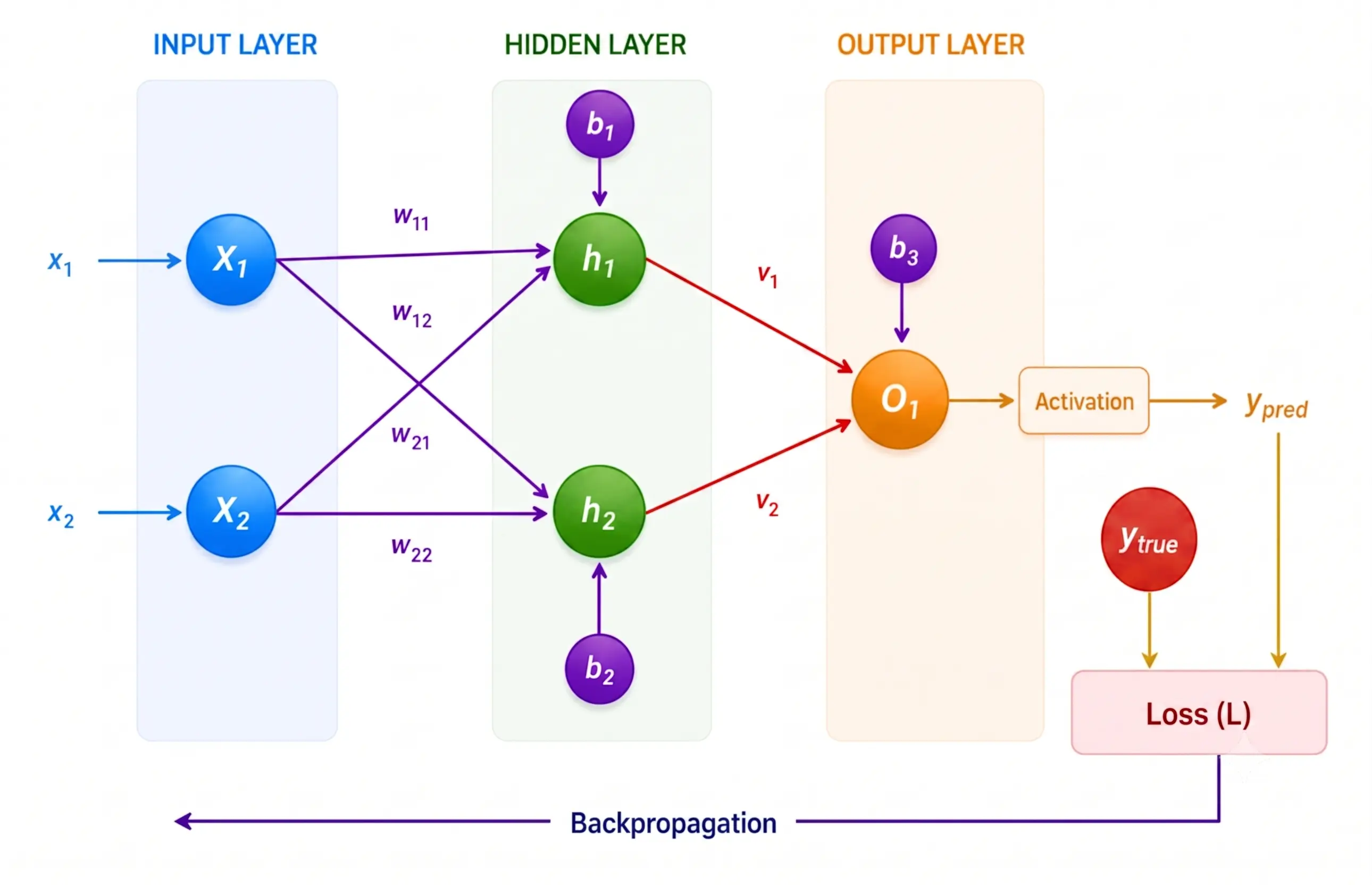
A typical ANN has an input layer which is the entry point of the structure. It receives input data and for every input value there is a node or neuron. No computation happens at the input layer.
Any real world ANN architecture has lots of hidden layers but here in the above diagram we considered only one layer for simplicity. The presence of many hidden layers makes the structure Deep. Hidden layers are intermediate computational layers that take the input from the input layer and send computed results to the output layer.
Output layer takes processed output from different last hidden layer, applies some transformation and generates the predicted output \(y_{pred}\).
$$ \text{Forward Pass: Input Layer} \to \text{Hidden Layer(s)} \to \text{Output Layer} $$
This process iterates over multiple times until we are able to generate a very good prediction compared to the actual value \(y_{true}\). This sums up the forward pass of ANN.
Now the obvious question is why do we repeat the forward pass. The answer is refinement of the prediction. How do we refine the prediction? Gradient descent mechanism to update the parameters that minimise the loss.
The Backward Pass
If we carefully look into the above diagram, we will notice that the loss captures the gap between true value and predicted value and depends only on the transformed value of \(O_1\). So, the loss will depend on the quality of \(O_1\). But \(O_1\) is not standalone; it also takes input from hidden layers which process input. So, the quality of \(O_1\) is dependent on \(h_1\) and \(h_2\) too. Since, output of one layer is fed to the next layer as input in the forward pass, there should be a mechanism to pass the loss from output layer to input; so that gradient of the loss can be calculated with respect to parameters - weights and biases of each layer so that parameters can be updated following gradient descent in each iteration. This backward flow of loss is called Backpropagation.
$$ \text{Backward Pass: Output Layer} \to \text{Hidden Layer(s)} \to \text{Input Layer} $$
Generally, every node computes a weighted sum and applies some transformations called Activations but here for simplicity we are showing activations only in the output layer.
Mathematically, the forward pass can be written as:
$$ h_1 = w_{11} \cdot x_1 + w_{21} \cdot x_2 + b_1 $$
$$ h_2 = w_{12} \cdot x_1 + w_{22} \cdot x_2 + b_2 $$
$$ o_1 = h_1 \cdot v_1 + h_2 \cdot v_2 + b_3 $$
$$ y_{pred} = f(o_1) $$
$$ \text{Loss } L = loss(y_{pred}, y_{true}) $$
Backpropagation starts from output layer as:
$$ \frac{\partial L}{\partial y_{pred}} = \frac{\partial}{\partial y_{pred}}\ loss(y_{pred}, y_{true}) $$
Since in the activation layer \(y_{pred} = f(o_1)\), we can use chain rule to calculate
$$ \frac{\partial L}{\partial o_1} = \frac{\partial L}{\partial y_{pred}} \cdot \frac{\partial y_{pred}}{\partial o_1} $$
$$ \frac{\partial y_{pred}}{\partial o_1} = f’(o_1) $$
In the output layer,
$$ \text{gradient with respect to } v_1: \quad \frac{\partial L}{\partial v_1} = \frac{\partial L}{\partial o_1} \cdot \frac{\partial o_1}{\partial v_1} = \frac{\partial L}{\partial y_{pred}} \cdot \frac{\partial y_{pred}}{\partial o_1} \cdot h_1 $$
$$ \text{gradient with respect to } v_2: \quad \frac{\partial L}{\partial v_2} = \frac{\partial L}{\partial o_1} \cdot \frac{\partial o_1}{\partial v_2} = \frac{\partial L}{\partial y_{pred}} \cdot \frac{\partial y_{pred}}{\partial o_1} \cdot h_2 $$
$$ \text{gradient with respect to } b_3: \quad \frac{\partial L}{\partial b_3} = \frac{\partial L}{\partial o_1} \cdot \frac{\partial o_1}{\partial b_3} = \frac{\partial L}{\partial y_{pred}} \cdot \frac{\partial y_{pred}}{\partial o_1} $$
In the hidden layer,
$$ \text{gradient with respect to } w_{11} \text{ for } h_1: \quad \frac{\partial L}{\partial w_{11}} = \frac{\partial L}{\partial o_1} \cdot \frac{\partial o_1}{\partial h_1} \cdot \frac{\partial h_1}{\partial w_{11}} = \frac{\partial L}{\partial y_{pred}} \cdot \frac{\partial y_{pred}}{\partial o_1} \cdot v_1 \cdot x_1 $$
$$ \text{gradient with respect to } w_{21} \text{ for } h_1: \quad \frac{\partial L}{\partial w_{21}} = \frac{\partial L}{\partial o_1} \cdot \frac{\partial o_1}{\partial h_1} \cdot \frac{\partial h_1}{\partial w_{21}} = \frac{\partial L}{\partial y_{pred}} \cdot \frac{\partial y_{pred}}{\partial o_1} \cdot v_1 \cdot x_2 $$
$$ \text{gradient with respect to } b_1 \text{ for } h_1: \quad \frac{\partial L}{\partial b_1} = \frac{\partial L}{\partial o_1} \cdot \frac{\partial o_1}{\partial h_1} \cdot \frac{\partial h_1}{\partial b_1} = \frac{\partial L}{\partial y_{pred}} \cdot \frac{\partial y_{pred}}{\partial o_1} \cdot v_1 $$
$$ \text{gradient with respect to } w_{12} \text{ for } h_2: \quad \frac{\partial L}{\partial w_{12}} = \frac{\partial L}{\partial o_1} \cdot \frac{\partial o_1}{\partial h_2} \cdot \frac{\partial h_2}{\partial w_{12}} = \frac{\partial L}{\partial y_{pred}} \cdot \frac{\partial y_{pred}}{\partial o_1} \cdot v_2 \cdot x_1 $$
$$ \text{gradient with respect to } w_{22} \text{ for } h_2: \quad \frac{\partial L}{\partial w_{22}} = \frac{\partial L}{\partial o_1} \cdot \frac{\partial o_1}{\partial h_2} \cdot \frac{\partial h_2}{\partial w_{22}} = \frac{\partial L}{\partial y_{pred}} \cdot \frac{\partial y_{pred}}{\partial o_1} \cdot v_2 \cdot x_2 $$
$$ \text{gradient with respect to } b_2 \text{ for } h_2: \quad \frac{\partial L}{\partial b_2} = \frac{\partial L}{\partial o_1} \cdot \frac{\partial o_1}{\partial h_2} \cdot \frac{\partial h_2}{\partial b_2} = \frac{\partial L}{\partial y_{pred}} \cdot \frac{\partial y_{pred}}{\partial o_1} \cdot v_2 $$
It is evident from the calculation that the gradient of loss with respect to parameter(s) of one layer is simply multiplication of chain of gradient of loss with respect to the final prediction in the output layer, gradient of loss with respect to the input to output layer and the gradient propagates back as gradient of loss with respect to output of any intermediate layer until it reaches the output of the current layer.
Finally the gradient descent algorithm is applied as -
$$ \text{For any weight } w, \quad w_{new} \leftarrow w - \eta \cdot \frac{\partial L}{\partial w} $$
$$ \text{For any bias } b, \quad b_{new} \leftarrow b - \eta \cdot \frac{\partial L}{\partial b} $$
Computation Graph
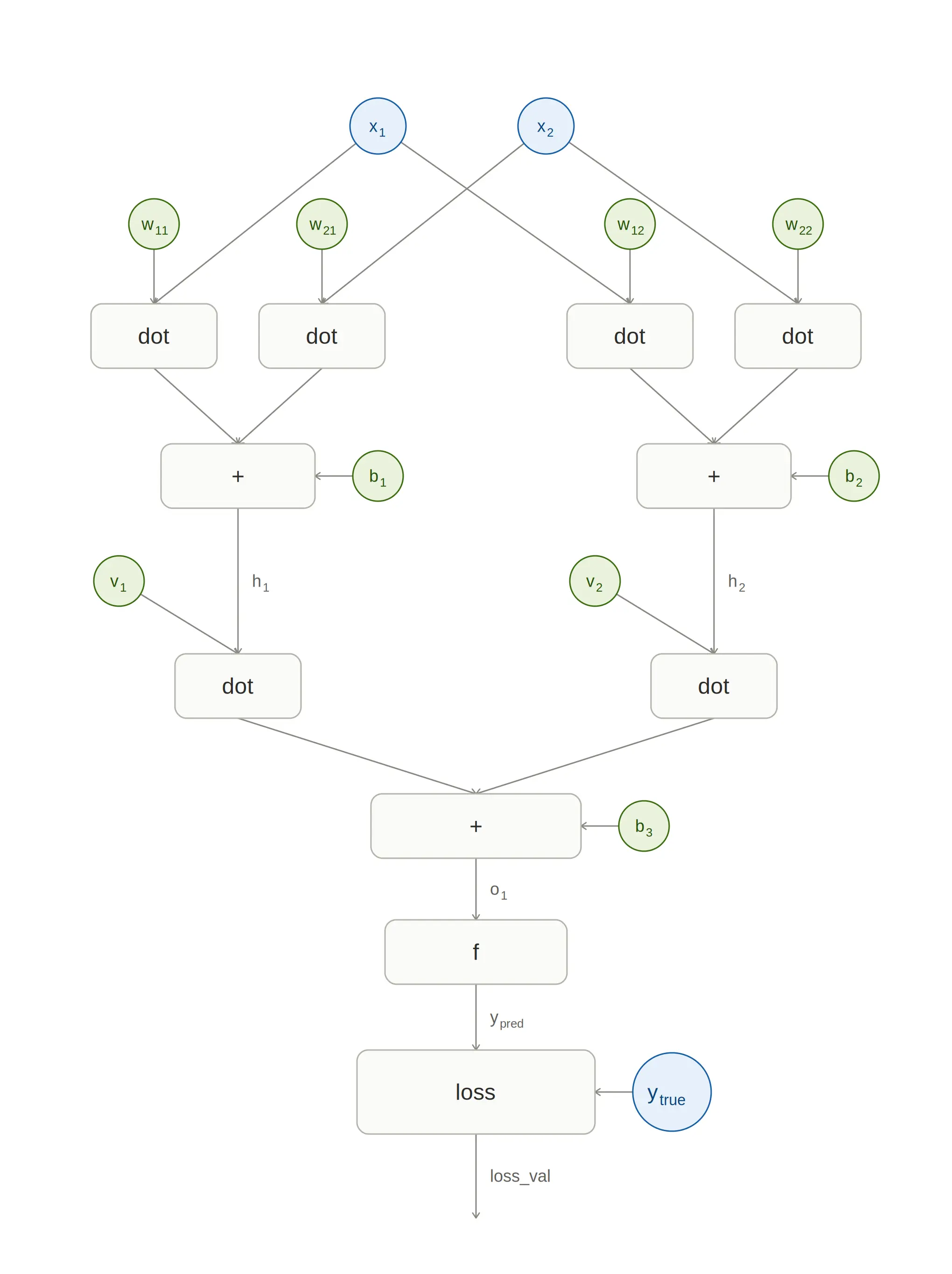
During forward pass, the computation graph of deep learning architecture is formulated. It captures the flow of data and mathematical operations involving them in the neural network. It isolates the independent operations that can be computed parallelly. This graph helps the optimization process understand how the data elements are linked with operations, what should be the backward flow and determine how the gradient to be calculated using chain rule.
Frameworks like Pytorch, Keras/Tensorflow use this computation graph during the forward pass and don’t actually calculate the gradient in the backward direction. This technique is called Automatic Differentiation.
Here is a small Python implementation of the above example assuming the function \(f\) as Sigmoid and the loss as mean squared error.
import torch
import torch.nn as nn

# Input and Target
X = torch.tensor([[0.5, 0.8]])
y = torch.tensor([[1.0]])

# Network: 2 → 2 (Linear) → 1 (Linear) → Sigmoid
model = nn.Sequential(
    nn.Linear(2, 2),
    nn.Linear(2, 1),
    nn.Sigmoid()
)

# Initialize weights and biases
with torch.no_grad():
    model[0].weight[:] = torch.tensor([[0.2, -0.3],
                                        [-0.4, 0.5]])
    model[0].bias[:] = torch.tensor([0.1, -0.2])
    model[1].weight[:] = torch.tensor([[0.3, -0.1]])
    model[1].bias[:] = torch.tensor([0.2])

loss_fn = nn.MSELoss()
optimizer = torch.optim.SGD(model.parameters(), lr=0.1)

print("Initial Parameters")
print("------------------")
for name, p in model.named_parameters():
    print(f"{name}\n{p.data}\n")

# Forward Pass
y_pred = model(X)
loss = loss_fn(y_pred, y)

# Backward Pass
optimizer.zero_grad()
loss.backward()
print("Gradients")
print("---------")
for name, p in model.named_parameters():
    print(f"{name}\n{p.grad}\n")

# Gradient Descent
optimizer.step()
print("Updated Parameters")
print("------------------")
for name, p in model.named_parameters():
    print(f"{name}\n{p.data}\n")
Its output is -
Initial Parameters
------------------
0.weight
tensor([[ 0.2000, -0.3000],
        [-0.4000, 0.5000]])
0.bias
tensor([ 0.1000, -0.2000])
1.weight
tensor([[ 0.3000, -0.1000]])
1.bias
tensor([0.2000])
Gradients
---------
0.weight
tensor([[-0.0337, -0.0539],
        [ 0.0112, 0.0180]])
0.bias
tensor([-0.0674, 0.0225])
1.weight
tensor([[0.0090, 0.0000]])
1.bias
tensor([-0.2246])
Updated Parameters
------------------
0.weight
tensor([[ 0.2034, -0.2946],
        [-0.4011, 0.4982]])
0.bias
tensor([ 0.1067, -0.2022])
1.weight
tensor([[ 0.2991, -0.1000]])
1.bias
tensor([0.2225])