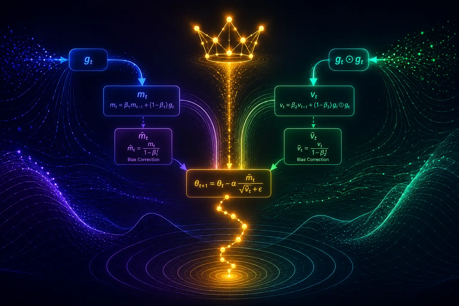
In part 5 we explored optimization strategies that ensure a solution to local optima problems and can navigate through flat saddle points. From the foundational approach of Gradient Descent we have moved to its refined version of Momentum based methods and techniques that involve Adaptive Learning Rate. These techniques, though advanced, have some bottlenecks. For example, the Momentum method can increase the momentum such that it can overshoot or oscillate in high curvature loss surfaces. AdaGrad has the potential to make the learning to almost stop when gradients are high, for RMSProp, if the data pattern is unstable then their gradient will be erratic and that will create uneven weight updated in different iterations.
ADAM Intuition
ADAM stands for Adaptive Moment Estimation and is another optimization strategy that combines best of momentum based and adaptive learning rate based algorithms. It is a de-facto lead in the world of optimization strategies for deep learning and is used extensively.
In general, it amalgamates momentum based methods by accumulating past gradients and adaptive learning rate mechanisms by customizing learning rate for each parameter.
First Moment
The first moment tracks the mean of the past gradients and, similar to RMSProp, uses an exponential decay of past gradients to control the history and makes the updates consistent.
If \(g\) is the current gradient, \(m\) stores the moving average (first moment) of the gradient, \(\beta_1\) is the exponential decay rate for the first moment and \(t\) defines the current timestep, then
$$ m_t = \beta_1 \cdot m_{t-1} + (1 - \beta_1) \cdot g_t $$
Second Moment
ADAM also captures the variance of the past squared gradients (second moment) and uses an exponential decay. The moving average of squared gradients controls the variation of step size by amplifying/shrinking the customized step size for each parameter as needed.
If \(g\) is the current gradient, \(v\) stores the moving average (first moment) of the squared gradient, \(\beta_2\) is the exponential decay rate for the second moment and \(t\) defines the current timestep, then
$$ v_t = \beta_2 \cdot v_{t-1} + (1 - \beta_2) \cdot g_t^2 $$
Bias Correction
Initially at \(t = 0\), \(m_0\) and \(v_0\) are initialized with 0, \(\beta_1\) and \(\beta_2\) have values close to 1; so when \(t\) is small, the first and second moments tend to zero due to lack of sufficient history and need a correction.
$$ \hat{m}_t = \frac{m_t}{1-\beta_1^t} $$
$$ \hat{v}_t = \frac{v_t}{1-\beta_2^t} $$
As \(t\) progresses, history starts building up and \(\beta_1\), \(\beta_2\) approaches to 0. So the denominator approaches to 1 and the effect of bias correction gets nullified.
Parameter Update
For parameter \(\theta\), learning rate \(\alpha\), smoothing term \(\epsilon\) and current timestep \(t\),
$$ \theta_t \leftarrow \theta_{t-1} - \frac{\alpha}{\sqrt{\hat{v}_t}+\epsilon} \cdot \hat{m}_t $$
The overall performance of ADAM - fast convergence, handling of noisy gradients and less hyperparameter tuning make it the crown jewel of the family of optimizers.
AdamW
AdamW is a variation of ADAM and it addresses a critical flaw in the architecture of the original ADAM optimizer. It is the standard optimizer for modern deep learning like Transformers and Large Language Models.
In vanilla gradient descent the update of the parameter is -
$$ \theta_{t+1} \leftarrow \theta_t - \alpha \cdot \nabla L(\theta_t) $$
But in reality, there is a \(L_2\) regularization that gets added to the loss function \(L\) where \(\lambda\) acts as the regularization parameter.
$$ L’(\theta_t) = L(\theta_t) + \frac{\lambda}{2}|\theta_t|^2 $$
So the actual gradient descent update will be
$$ \theta_{t+1} \leftarrow \theta_t - \alpha \cdot \nabla L’(\theta_t) $$
$$ \theta_{t+1} \leftarrow \theta_t - \alpha \cdot \nabla\left(L(\theta_t) + \frac{\lambda}{2}|\theta_t|^2\right) $$
$$ \theta_{t+1} \leftarrow \theta_t - \alpha \cdot \nabla L(\theta_t) - \alpha \cdot \lambda \cdot \theta_t $$
$$ \theta_{t+1} \leftarrow (1 - \alpha \cdot \lambda)\theta_t - \alpha \cdot \nabla L(\theta_t) $$
From the above equation it is evident that there is a weight decay part \((1 - \alpha \cdot \lambda)\) in addition to standard gradient descent.
For optimizers like ADAM, the design is exactly the same with gradient descent - passing the regularization part \(\frac{\lambda}{2}|\theta|^2\) directly into the loss function.
So the actual gradient \(g\) at timestep \(t\) is:
$$ \hat{g}t = g_t + \lambda \cdot \theta{t-1} $$
If we look into the calculation of \(\hat{m}_t\) and \(\hat{v}_t\), we can infer that the true gradients of model parameters and gradients of regularization terms both get mixed up. So, instead of considering only the parameter gradients, regularization gradients are also kept in the parameter update logic.
The revised update rule considering \(L_2\) regularization,
$$ \theta_t \leftarrow \theta_{t-1} - \frac{\alpha}{\sqrt{\hat{v}_t}+\epsilon} \cdot \hat{m}_t $$
$$ \theta_t \leftarrow \theta_{t-1} - \frac{\alpha \cdot (\beta_1 \cdot m_{t-1} + (1-\beta_1) \cdot (g_t + \lambda \cdot \theta_{t-1}))}{\sqrt{\hat{v}_t}+\epsilon} $$
$$ Update \propto \frac{(g_t + \lambda \cdot \theta_{t-1})}{\sqrt{\hat{v}_t}+\epsilon} $$
So, when historical gradients are high, \(\sqrt{\hat{v}_t}\) is also large and the regularization part is divided by a large number and the effective penalty becomes small. Conversely, when historical gradients are low, \(\sqrt{\hat{v}_t}\) is small and the regularization part is divided by a small number and the effective penalty becomes amplified.
AdamW Parameter Update
To fix the aforementioned issue, AdamW has a revised update rule where the regularization part is decoupled from the parameter gradient section and the regularization gradient i.e. weight decay part is not scaled by \(\sqrt{\hat{v}_t}\) and does not get distorted.
$$ \theta_t \leftarrow \theta_{t-1} - \alpha \cdot \lambda \cdot \theta_{t-1} - \frac{\alpha}{\sqrt{\hat{v}_t}+\epsilon} \cdot \hat{m}_t $$