
In today’s world, Artificial Intelligence (AI) can do magic. You ask questions to a chatbot, it responds in seconds. Once we watch a web-series on Netflix, similar series are automatically recommended. The same goes for YouTube. Think about biometric authentication, in a split of a second the application is able to detect someone as an imposter. Once we initiate a credit card application online, within seconds it shows the creditworthiness of the applicant. Do you think somebody is there or some application is written with specific rules? Absolutely not! These are all data driven decisions where the outcome is generated from data interaction and pattern recognition.
So, the crux is data and data representation such that any AI application can identify patterns for effective insights from it.
The Secret Language of AI
For most people, AI or traditional Machine Learning is like a black box where maximum processing is hidden. In this six-part series we will try to unearth some of the secrets.
Since we need to deal with different forms of data at different scales, their interaction and the transformation of that data during pattern recognition, one of the primary secret sauce of AI is Linear Algebra because it provides the mathematical framework that defines those interactions. It is that branch of Mathematics where data gets changed in a linear predictable way by application of some functions. If we plan to get to the bottom of how AI systems learn we need to grasp the fundamental concepts of Linear Algebra that explain the Geometry formed by the data representation.
Turning Reality into Numbers
For face based authentication when the app captures the image, it does not treat it as a separate image object; rather it treats it as a grid of numbers. Similarly, every user profile in Netflix or YouTube is maintained as a grid of numbers. To check creditworthiness we need demographic and financial details of the applications, all are again a set of numbers. If there are categorical attributes we convert it to meaningful numbers. Each word of our question to a chatbot also has a numerical representation. The data can be tabular i.e. structured or it can be of unstructured type; but irrespective of that it is just a set of numbers to the AI application which will use that data, learn patterns and be able to make future predictions.
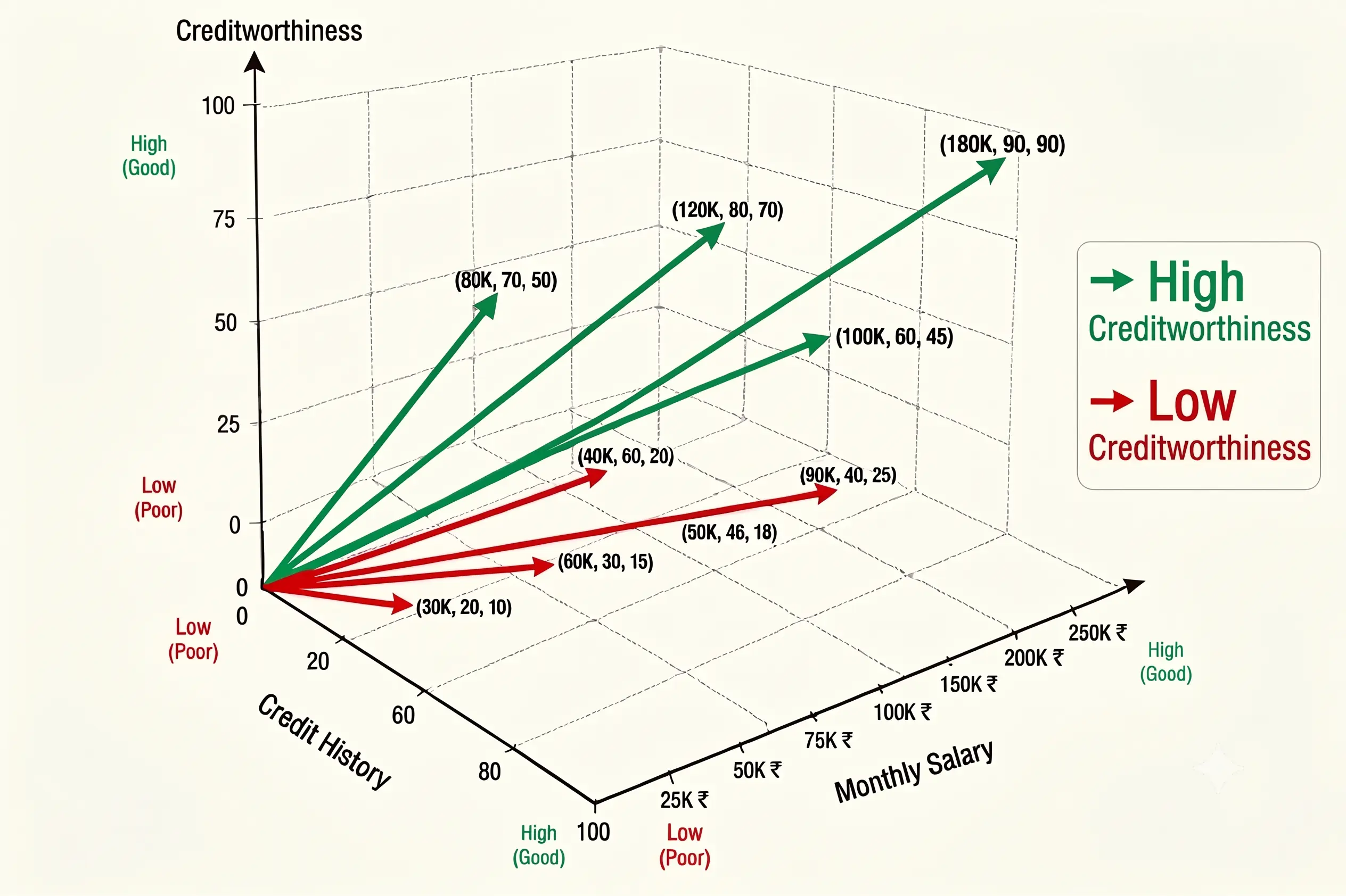
In the simplest form, the numerical attributes of each observation produces a vector in a multi-dimensional space where each dimension represents one attribute.
As you can see in the 3-D image below, monthly salary and credit history represented in x and y axes are determining factors of creditworthiness shown in z-axis. So, for each vector of length two constituted of monthly salary and credit history of each applicant there is a creditworthiness score and together they form a three dimensional representation for each observation and we can say each applicant is numerically embedded in a three dimensional vector.
The Building Blocks of Data
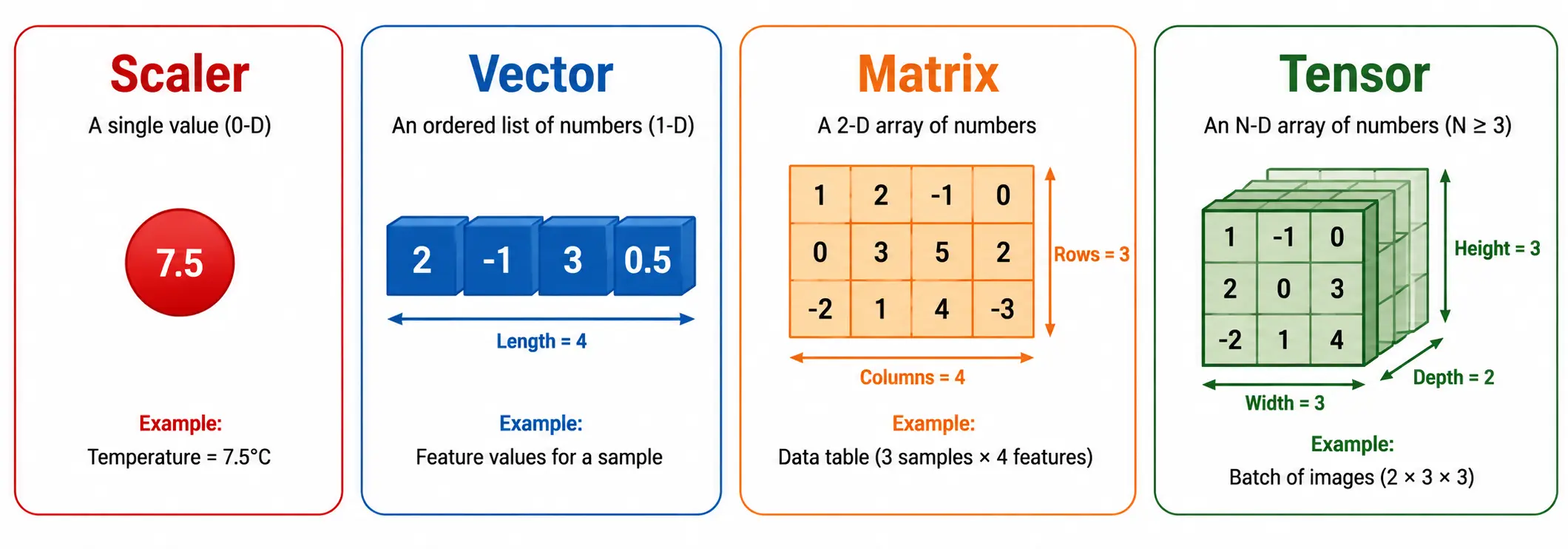
When we talk about data, it can be of four forms internally -
- Scaler: Any numerical value without any direction such as credit history of an applicant or temperature.
- Vector: A set of numerical values representing an object such as credit history, monthly salary and creditworthiness of an applicant. It has a direction.
- Matrix: If a credit applicant has 3 attributes and if we have 100 applicants then the overall dataset of 100 rows and 3 columns is called a matrix.
- Tensor: This is a multi-dimensional array that looks like matrices stacked together. It has specific use in Deep Learning where batches of images are processed together. If an image is has dimension of \(m * n\) and each batch has \(b\) images then the stacked matrix has dimension \(b * m * n\). Tensor generalizes the internal data formats where scaler is rank-0, vector is rank-1 and matrix is rank-2 tensors respectively.
Living in High-Dimensional Space
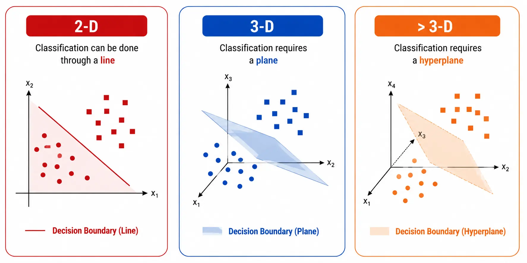
We mentioned earlier that each attribute or feature of an observation defines an axis. So, if there are \(n\) features then technically there are \(n\) dimensions and \(n\) axes forming the Feature Space. This fact brings the concept of multi-dimensionality in AI applications. There can be few dimensions out of \(n\) that are more dominant and there are techniques to identify those specific dimensions. When we apply some function for data transformation, it has to be aligned with the data dimension. For example, classification in 2-D can be done through a line, in 3-D we need a plane and for more than 3-D we need a hyperplane.
Vector Addition and Scaling
Vector addition signifies summation of two vectors or subtraction of one vector from another provided they both have the same dimension. The resultant vector has a completely different magnitude and direction from its constituents.
It’s like subtracting the man vector from the king vector and adding the woman vector resulting in the vector for queen.
Scaling on the other hand, is multiplication of all the elements of a vector by a scaler. The resulting vector will have a different magnitude in the same direction of the original vector. A simple example can be multiplying all values in the matrix of an image by a fixed scalar number.
Understanding Magnitude
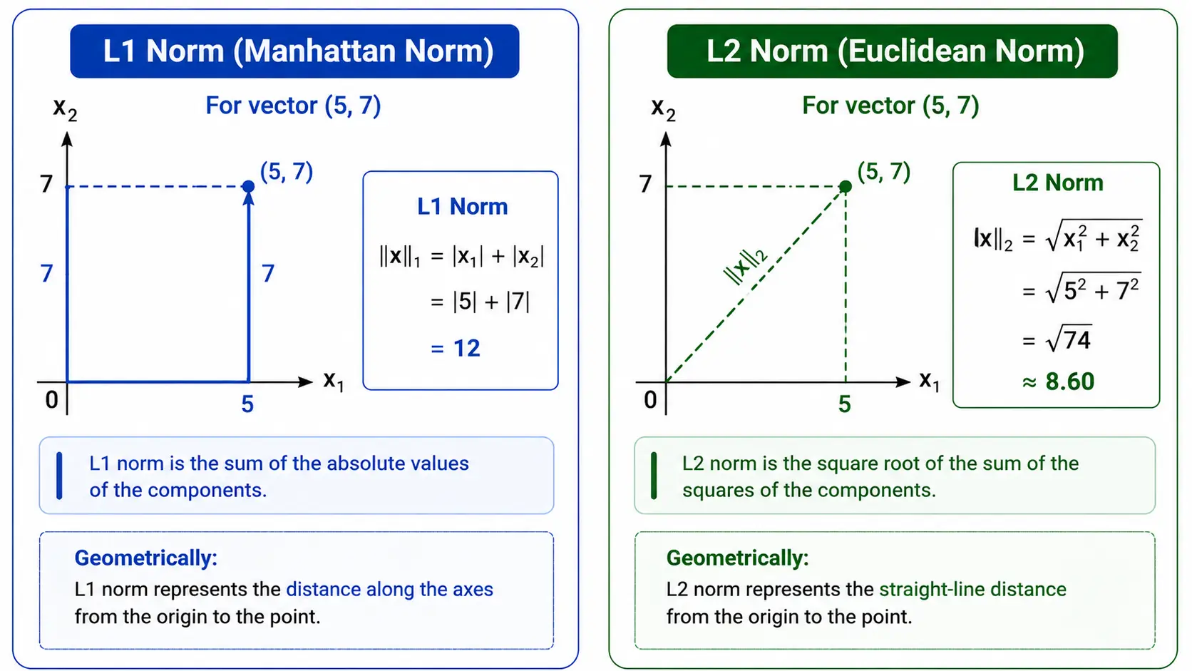
During the pattern recognition phase of an AI algorithm, it deals with a lot of vectors of each observation and the vectors are of different length. To avoid numerical instability it is required to bring them within the same range through a process called Feature Scaling or Normalization and at that time the length i.e. the magnitude of the vector needs to be calculated.
The most popular techniques are -
- L1-Norm: For a \(n\) dimensional vector \(X\), it is the sum of absolute values of individual components.
$$ ||X||_1 = |x_1| + |x_2| + … + |x_n| $$
- L2-Norm: For a \(n\) dimensional vector \(X\), it is the square root of the sum of squared values of individual components.
$$ ||X||_2 = \sqrt{x_1^2 + x_2^2 + … + x_n^2} $$
Distance Between Data Points
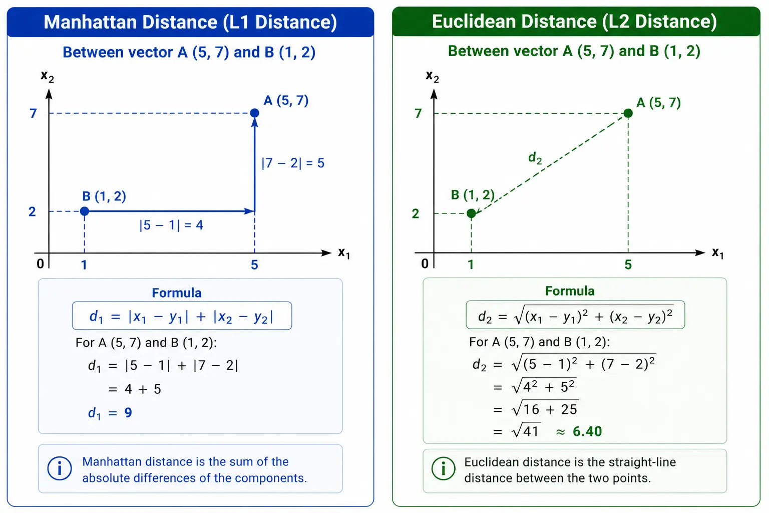
The observations which are close enough in terms of their attributes must have similar numerical values for their attributes. That means the vectors they form are also close to each other. So, if we measure the closeness of two vectors through calculating the distance between them, we can easily determine if those two vectors are similar or not. If they are similar, the distance between them will be close to zero.
The common techniques are -
- Manhattan Distance: For two \(n\) dimensional vectors \(X\) and \(Y\), it is the sum of absolute differences of individual components. It can be construed from the definition of L1-norm that it calculates the distance from origin and it is almost the same as Manhattan distance.
$$ d_1 = |x_1 - y_1| + |x_2 - y_2| + … + |x_n - y_n| $$
- Euclidean Distance: For a \(n\) dimensional vector \(X\) and \(Y\), it is the square root of the sum of squared differences of individual components. It is also similar to L2-norm if we consider origin as one vector.
$$ d_2 = \sqrt{(x_1 - y_1)^2 + (x_2 - y_2)^2 + … + (x_n - y_n)^2} $$
Direction Matters More
In reality when we ask a question to a chat bot and use a specific phrase in our question, we may have noticed that the chat bot responds using similar phrases which have Semantic Similarity to the original phrase. Sometimes we need to find out if two vectors are pointing in the same direction or how they are aligned with each other. It is particularly important when vectors have small magnitudes; so their distance is also very small but they may point in different directions. So, distance alone is not the ultimate decider of vector similarity.
The metric to measure the direction is called Dot Product. It is defined as the product of L1-norm or the length of individual vectors \(X\) and \(Y\) and the cosine of the angle between them.
$$ dot(X, Y) = ||X||_2 \cdot ||Y||_2 \cdot Cos(\theta) $$
If vectors \(X\) and \(Y\) are defined as \([x_1, x_2, …, x_n]^T\) and \([y_1, y_2, …, y_n]^T\) respectively, then
$$ dot(X, Y) = (x_1 * y_1) + (x_2 * y_2) + … + (x_n * y_n) $$
The dot product generates a scalar value, where positive value indicates the same direction, negative value indicates opposite direction. When dot product is zero then vectors are unrelated with each other which is possible if the angle between them is \(90°\) because \(Cos(90°) = 0\) and two vectors are said to be Orthogonal. Conversely, if the dot product between two vectors is zero then they are also said to be Orthogonal.
Here are some of the important properties of dot product -
- Distributive: \((u + v) \cdot w = u \cdot w + v \cdot w\) where \(u, v, w\) are vectors.
- Commutative: \(u \cdot v = v \cdot u\)
- Scaler Multiplication: \(ku \cdot v = k * (u \cdot v) = u \cdot (kv)\)
From the formula for dot product it is evident that it gets affected by the magnitude of vectors. So, if we want to understand the direction by measuring the angle between the vectors then the metric is called Cosine Similarity ranging between \(-1\) to \(+1\) and it is defined as -
$$ Cosine\ Similarity\ (X, Y) = \frac{dot(X, Y)}{||X||_2 \cdot ||Y||_2} $$
You can check dot product and cosine similarity of different vectors in this simulation.