In the first blog we discussed how vectors represent data where the tip of the vector is a point in a multi-dimensional feature space. A vector, matrix or tensor represent different forms of data as input in a multitude of Artificial Intelligence (AI) algorithms. In the pattern identification process of each algorithm the raw data is transformed linearly multiple times to bring in desirable formats. The transformation may include rotating, stretching, reducing the dimensions and many more to extract insights from the data. One of the important connectors of Linear Algebra and AI is the Matrix that drills the theoretical transformations down to reality both physically and visually.
Linear Transformation
We have used this term multiple times without formally defining it. A transformation will be called linear if -
- The before to after translation is linear.
- The position of origin remains fixed.
Why the Matrix?
Basic to complex AI algorithms deal with tabular data of observations in row and attributes in columns. If we consider one column, it’s a vector; otherwise it is a matrix and if we stack multiple matrices then it is a tensor.
Let’s think about below scenario - where vector \([-5, 7]^T\) is transformed to \([5, 7]^T\). The transformation is linear because lines parallel to x and y axes remain parallel after transformation and the position of origin did not change. This transformation is possible with the application of a rectangular grid of numbers famously known as Matrix.
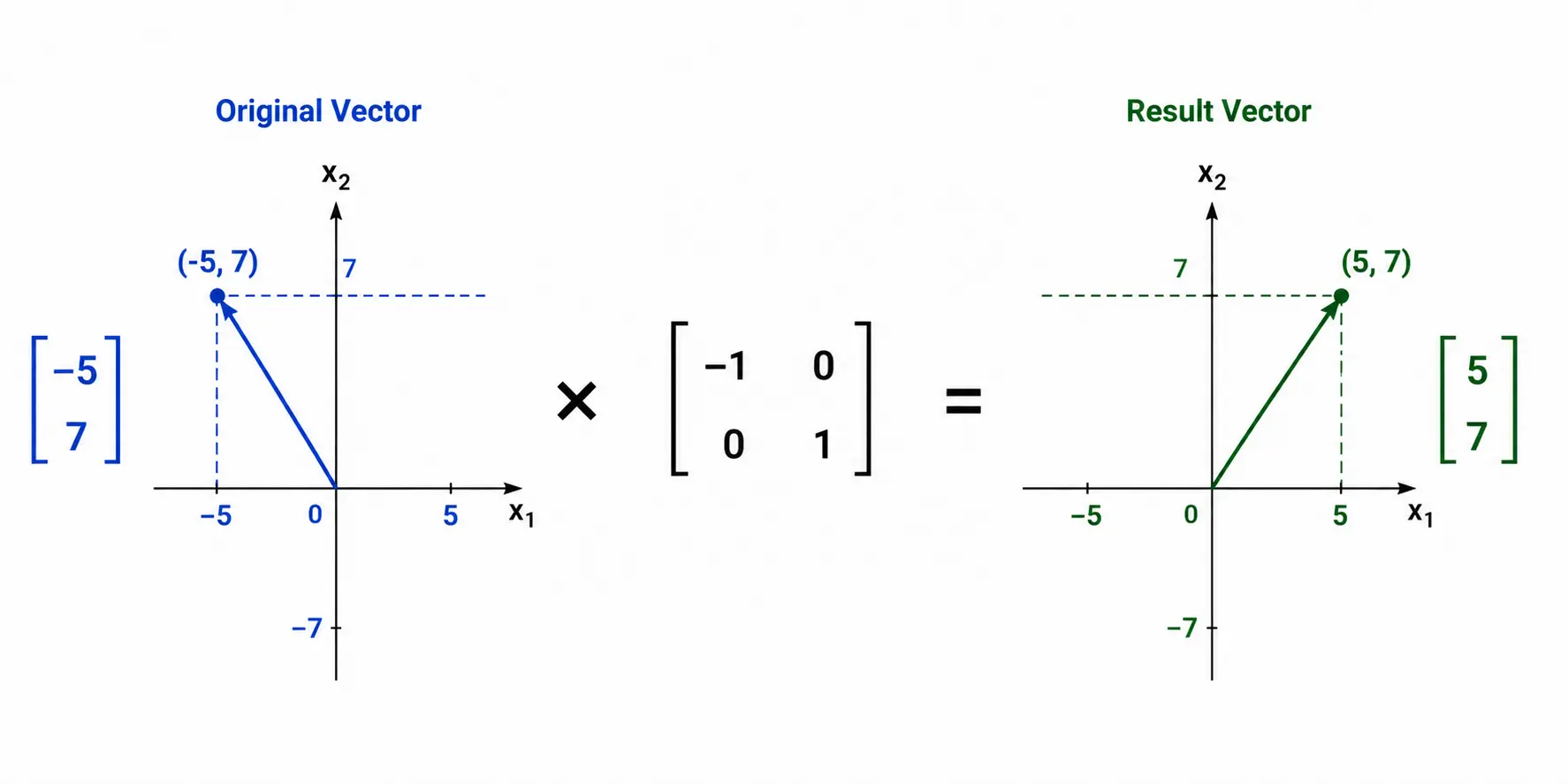
So the flipping of the vector is the result of a matrix operation and thus the matrix becomes an entangled part of modern AI.
Matrix Multiplication
Practically every linear transformation can be expressed as a matrix operation and complicated operations can be decomposed into a chain of matrix transformations.
There are few important properties of matrix (\(A, B, C\)) multiplication -
- Commutative: \(A * B \neq B * A\)
- Associative: \(A * (B * C) = (A * B) * C\)
- Distributive: \(A * (B + C) = A * B + A * C\)
The following interactive animation shows different types of linear transformations.
Solving Linear Equations
Why on earth are we discussing this here? Let’s take an example:
A house with 2,000 sq. ft. floor with 2 rooms costs 3 million INR and another house with 2,000 sq. ft. floor but with 1 room costs 2.5 million INR and we want to create a machine learning model to predict the price of the house if we supply its floor area and number of rooms.
The problem can be expressed through a set of linear equations; a solution to which is actual machine learning.
$$ 2W_1 + 2W_2 = 3 $$
$$ 2W_1 + W_2 = 2.5 $$
So, these 2 observations become the input to the machine learning model training process.
The input matrix can be written as:
| Floor Area (in 1,000 sq. ft.) | # of Rooms |
|---|---|
| 2 | 2 |
| 2 | 1 |
The output vector is:
| Price (in Million INR) |
|---|
| 3.0 |
| 2.5 |
The objective of any machine learning algorithm is to use below feature matrix \(A\) -
$$ \begin{bmatrix} 2 & 2 \\ 2 & 1 \end{bmatrix} $$
and find out the vector for model weights \(W = [w_1, w_2]^T\) such that
$$ A * W = Price $$
Equivalently, \(W = A^{-1} * Price\)
Or in standard notation,
$$ A\mathbf{X} = b \Rightarrow \mathbf{X} = A^{-1}b $$
The analogy above proves that bringing insights from features using an algorithm is actually finding out the solution of a system of linear equations by multiplying the inverse of the feature matrix with the label (Price) of observations and so existence of the inverse of the feature matrix is very crucial.
For a square matrix \(A\),
- If there exists another matrix \(B\) of same size, such that \(A * B = B * A = Identity\ Matrix\), then \(A\) is Invertible.
- Otherwise \(A\) is Non-Invertible or Singular.
Determinant of A Transformation
When we apply some linear transformations by means of matrix operations, the space covered by the vectors increase, decrease, can become positive, negative or even zero. The factor by which this area gets changed is called the Determinant of the matrix used in linear transformation.
Let’s take one example where original vector is:
$$ \begin{bmatrix} 1 & 0 \\ 0 & 1 \end{bmatrix} $$
where the space covered by the vectors is 1. If we apply different transformations as per below image we will get different resultant vectors where the factor by which the space covered by them in each scenario is changed is exactly the same as the determinant of the transforming 2×2 matrix calculated as below.
$$ \det\begin{bmatrix} a & b \\ c & d \end{bmatrix} = a * d - b * c $$
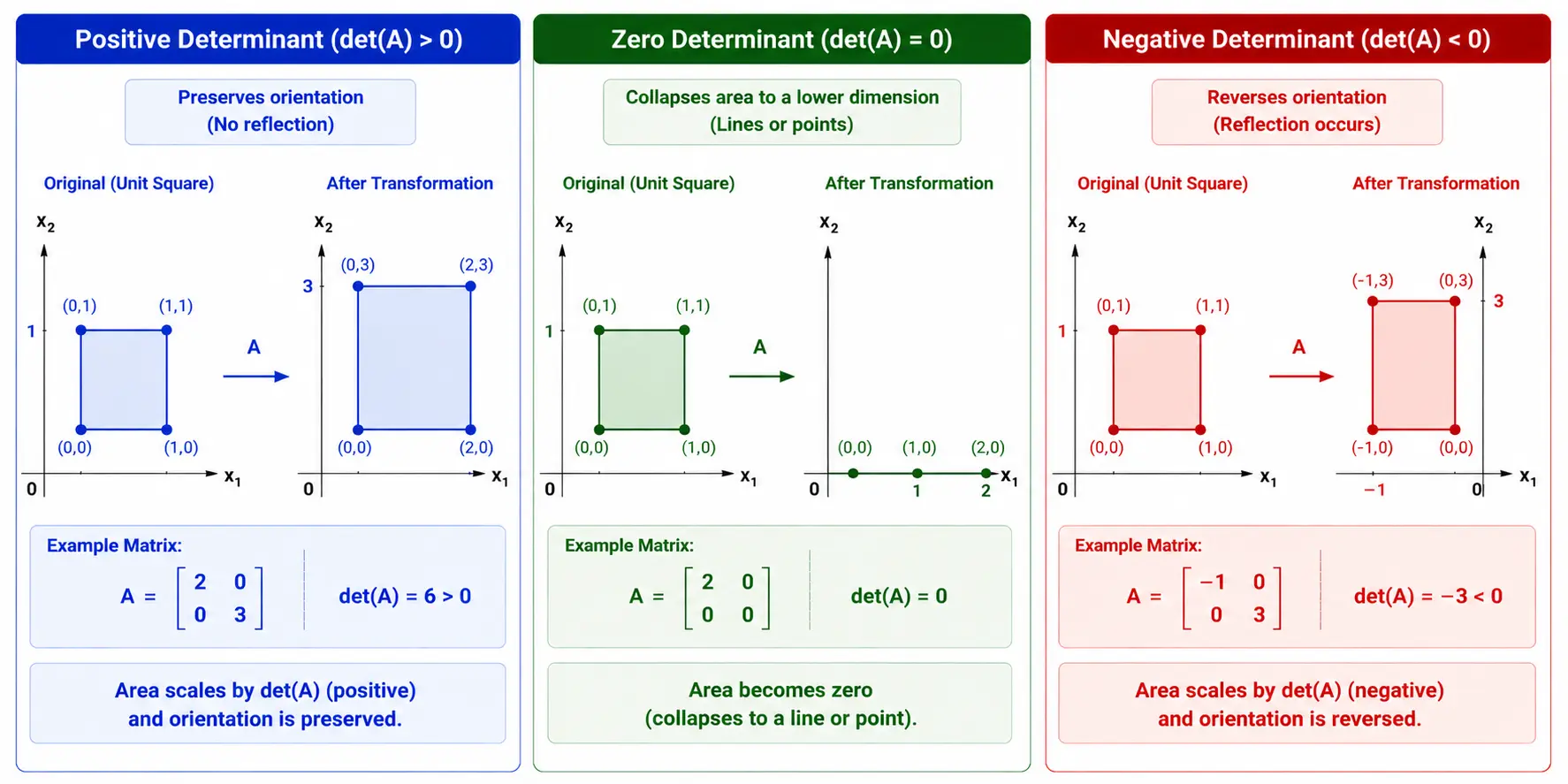
Determinant can be positive signifying the same orientation as was originally, negative signifying negative orientation compared to original or 0 means collapsing to a lower dimension. Determinant 1 means the orientation and space covered remains as it was before transformation.
The following important properties for determinant hold -
- For matrices \(u\) and \(v\), \(det(u, v) = -det(v, u)\).
- \(det(Matrix_1 \cdot Matrix_2) = det(Matrix_1) * det(Matrix_2)\).
- If \(det(Matrix\ A) = 0\) then matrix \(A\) is Non-Invertible or Singular means No Inverse Exists.
Since we are dealing with the feature matrix and if its determinant is non-zero, then the inverse matrix exists and we can reverse transform to get the original matrix. We will also have a unique solution to the system of equations and the ML algorithm output will be stable.
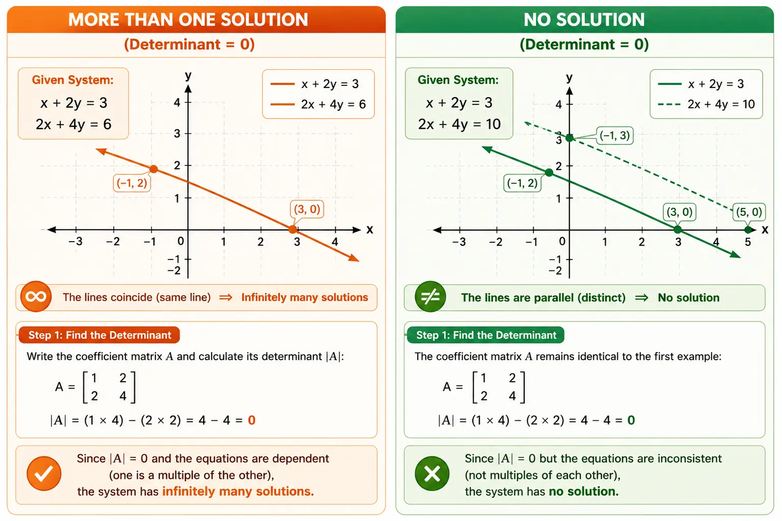
But if determinant is 0 then the original space coverage is flattened and we cannot get the original feature matrix back. From the system of linear equations perspective, there can be no solution or more than one solution and the ML algorithm will give an unstable, degenerate solution.