In blog 1, we discussed data representations. In blog 2 we talked about data transformations. We can process a plethora of information but having a lot of features does not necessarily mean that the Artificial Intelligence (AI) or Machine Learning (ML) model will be very powerful, rather the quality of the input data, specifically the uniqueness of each attribute, determines the quality of the machine learning and future predictions. The properties of transformed representations or transformed feature space helps the ML algorithm learn the real patterns of the feature space effectively.
The Concept of Vector Space
We mentioned earlier that numerical values of all attributes of any observation of any object such as all attributes of a person applying for a credit card/loan or the pixel values of an image forms a vector where each attribute defines a direction or axis. So, the set of vectors of all observations forms a feature space called Vector Space and the job of the algorithm is to find patterns, similarities etc. within that space.
Let \(u, v, w\) be vectors in the set \(V\). The set \(V\) is called vector space if following ten axioms are satisfied.
- Commutative: \(u + v = v + u\)
- Associative: \((u + v) + w = u + (v + w)\)
- Neutral Element: \(u + 0 = u\); 0 is zero vector
- Additive Inverse: \(u + (-u) = 0\)
- Closure under Vector Addition: \(u + v\) should also be in \(V\)
- Closure under Scalar Multiplication: \(ku\) should also be in \(V\); \(k\) is a scalar
- Associative: \(k \cdot (c \cdot u) = (k \cdot c) \cdot u\)
- Distributive Law for Vectors: \(k \cdot (u + v) = k \cdot u + k \cdot v\)
- Distributive Law for Scalars: \((k + c) \cdot u = k \cdot u + c \cdot u\)
- Identity Element: \(1 \cdot u = u\)
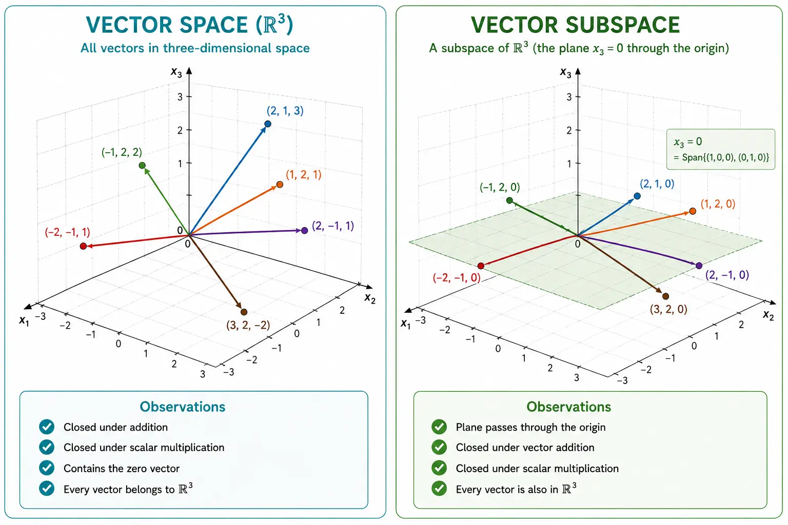
A non-empty subset consisting of a specific set of vectors chosen from \(V\) is called Vector Subspace and it also needs to satisfy ten axioms detailed above. During image compression, reducing features and selecting most effective ones, the entire search space for the AI/ML algorithm is reduced from vector space to vector subspace.
Here is an example of reducing dimensions using feature engineering.
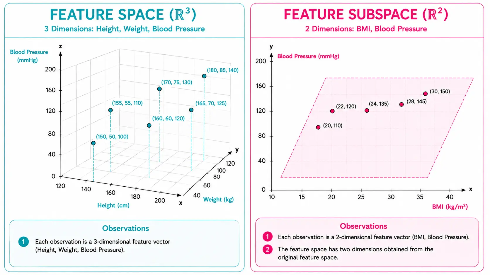
For a true vector space to subspace conversion this example shows how we can achieve that by making the 3rd dimension as zero.
Linear Independence
Let’s consider the task to predict the price of a house and think of a scenario where floor area both in square feet and square meter are available. Do you think using both of them makes any sense? Certainly not because the foot to meter conversion factor is fixed and so, one feature can be retrieved from another. This is an example of Linear Dependence. When all attributes are unique and cannot be deduced from another then they are Linearly Independent.
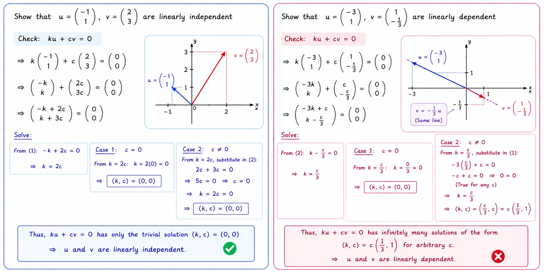
Mathematically, for a set of vectors \(v_1, v_2, …, v_n\) in \(\mathbb{R}^n\) or general vector space are linearly independent when for a set of scalars \(k_1, k_2, …, k_n\),
their linear combination \(k_1 \cdot v_1 + k_2 \cdot v_2 + … + k_n \cdot v_n = 0\) is possible if scalars \(k_1 = k_2 = k_n = 0\).
In summary,
- Linear combination of vectors is zero and only scalars are zero ⇒ Linear independence of all vectors.
- Linear combination of vectors is zero and any vector is zero ⇒ Linear dependence of all vectors.
Here are examples of linear independence and dependence.
Span of Vector
Take one vector as a sample, \(v = [4, 5]^T\).
It can be written as
$$ 4 \cdot \begin{bmatrix} 1 \\ 0 \end{bmatrix} + 5 \cdot \begin{bmatrix} 0 \\ 1 \end{bmatrix} $$
So, vector \(v\) can be expressed as a linear combination of \([1, 0]^T\) and \([0, 1]^T\).
Formally, the set of vectors that can be produced by linear combination i.e. vector addition and/or scalar multiplication of a set of vectors forms the Span of those vectors. For example, \([1, 0]^T\) and \([0, 1]^T\) span the entire \(\mathbb{R}^2\).
Basis - The Smallest Set
The set of vectors (\([1, 0]^T\) and \([0, 1]^T\) in the example above) that spans a vector space are called Basis or Spanning Set.
Theoretically, if \(v = {v_1, v_2, …, v_n}\) in \(\mathbb{R}^n\) forms a basis if
- \(v_1, v_2, …, v_n\) are linearly independent.
- \(v_1, v_2, …, v_n\) are generating set or spans \(\mathbb{R}^n\).
Here are some of the properties of basis -
- Any \(n\) linearly independent vectors in \(\mathbb{R}^n\) form a basis in \(\mathbb{R}^n\).
- Any \(n\) vectors which span \(\mathbb{R}^n\) form a basis for \(\mathbb{R}^n\).
The numerical examples below illustrate this concept.
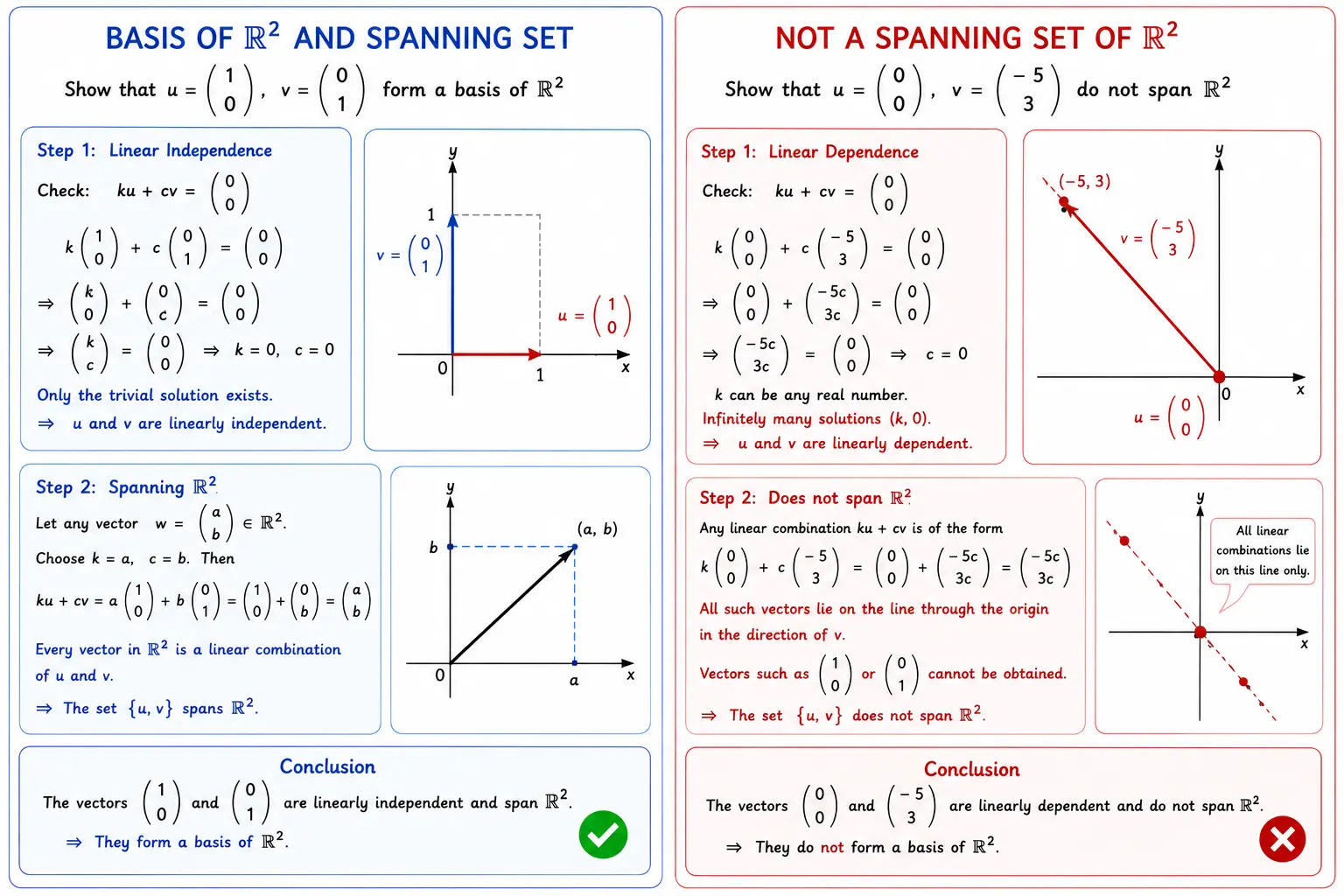
In AI/ML application, the endeavour should be finding out those attributes only that span the feature space because they capture the relationship well and reduce redundancy.
Some useful facts regarding basis are -
- A basis for a vector space is the largest independent set of vectors.
- A basis for a vector space is the smallest spanning set of vectors.
- Every vector can be written as a unique combination of basis vectors.
- In case of linear dependence, a vector can be expressed as a linear combination of other vectors.
Linear Transformation via Basis Vectors
Consider this linear transformation of flipping a vector from blog 2.
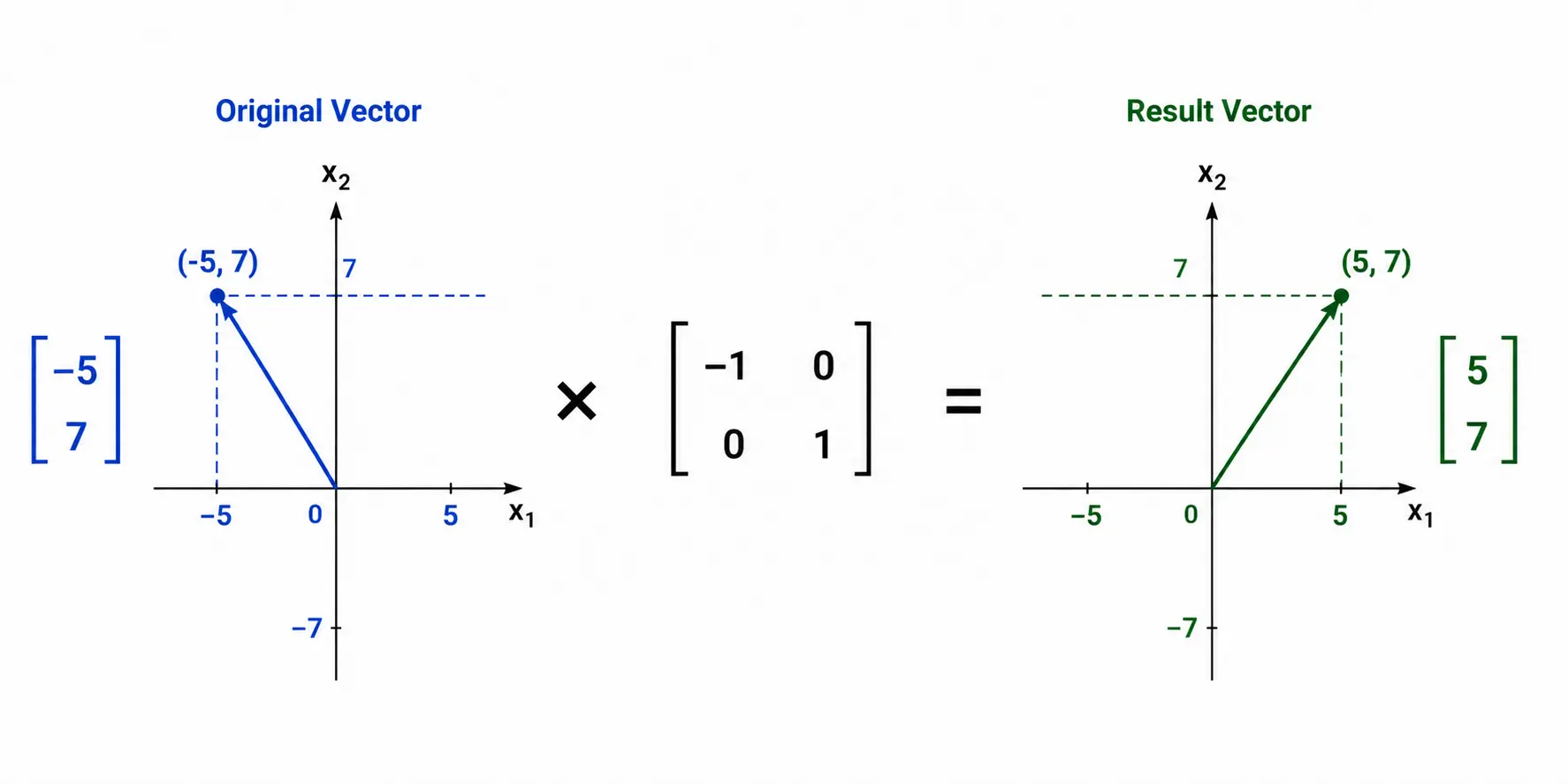
The original vector \(v = [-5, 7]^T\) can be written as -
$$ v = -5 \cdot \begin{bmatrix} 1 \\ 0 \end{bmatrix} + 7 \cdot \begin{bmatrix} 0 \\ 1 \end{bmatrix} $$
So, when we apply some linear transformation \(T\) on vector \(v\), it becomes
$$ T(v) = T\left(-5 \cdot \begin{bmatrix} 1 \\ 0 \end{bmatrix} + 7 \cdot \begin{bmatrix} 0 \\ 1 \end{bmatrix}\right) $$
$$ \Rightarrow T(v) = -5 \cdot T\left(\begin{bmatrix} 1 \\ 0 \end{bmatrix}\right) + 7 \cdot T\left(\begin{bmatrix} 0 \\ 1 \end{bmatrix}\right) $$
$$ \Rightarrow T(v) = -5 \cdot \begin{bmatrix} -1 \\ 0 \end{bmatrix} + 7 \cdot \begin{bmatrix} 0 \\ 1 \end{bmatrix} $$
$$ \Rightarrow Transformed\ v = \begin{bmatrix} 5 \\ 7 \end{bmatrix} $$
We can conclude that original basis vector \([1, 0]^T\) is transformed to \([-1, 0]^T\) and another original basis vector \([0, 1]^T\) remain unchanged. So, linear transformation of any vector or matrix is simply the shift of original basis vectors.
In summary,
\(Original\ Vector = Scalar\ Coefficients \times Original\ Basis\ Vectors\)
\(Transformed\ Vector = Scalar\ Coefficients \times Transformed\ Basis\ Vectors\)
The Uniqueness of Data - Rank
The matrix of observations and attributes may have \(n\) columns but all of them could potentially be not independent. Dimension captures the number of basis vectors needed to describe the vector space e.g. \(Dim(x-axis) = 1\).
Rank determines the number of linearly independent row or column vectors of the feature matrix. A matrix is Full-Rank if all attributes are linearly independent. Row Rank specifies the number of non-zero rows in row echelon form whereas Column Rank signifies the number of linearly independent attributes.
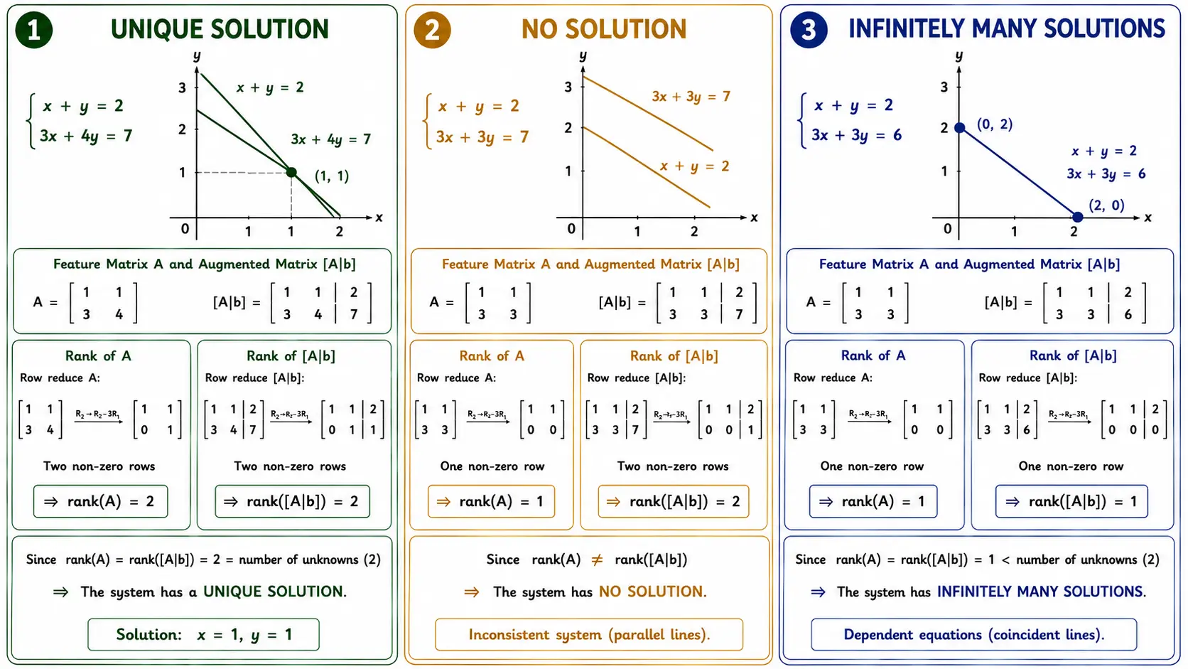
The rank of a feature matrix and the solution to the underlying system of linear equations that the matrix represents has a direct connection.
The standard form of linear equations is \(A\mathbf{X} = b\) where \(A\) is the feature matrix and \(A|b\) is the augmented matrix where the vector of the right hand side of the equations is appended as an additional column with the feature matrix. There can be three possibilities that can happen -
- \(Rank(A) = Rank(A|b) \Rightarrow\) Unique solution.
- \(Rank(A) \neq Rank(A|b) \Rightarrow\) No solution.
- \(Rank(A) = Rank(A|b) < n \Rightarrow\) Infinitely many solutions. Here the matrix is not full-rank and there are Free Variables defined as \(n - rank(A)\).
The mathematical example below depicts these three scenarios.