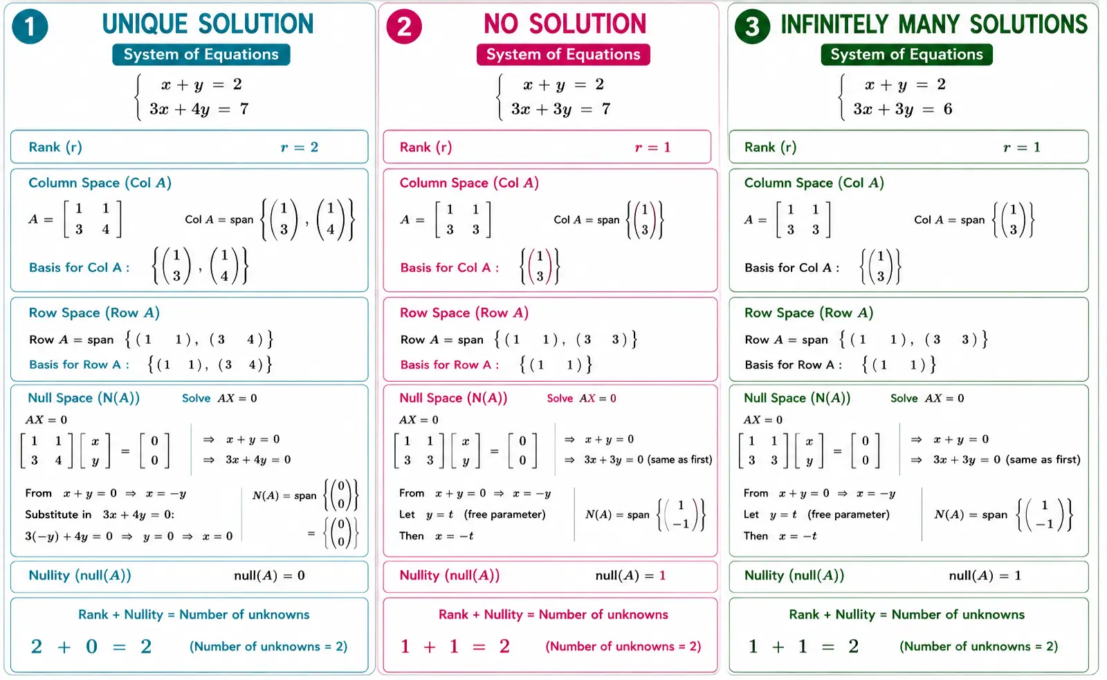
Previously, we looked at how data is represented and how matrix operations transform data. We talked about the structural components of attributes and explained that not all attributes make meaningful contributions to the process of learning of AI/ML algorithms. We mentioned solving a system of linear equations several times without formally defining the techniques and it’s now the time to do that. Additionally, there are four fundamental shorter geometric regions called Subspace inside the larger vector space and we need to know their connection to the solution of the system of linear equations.
Gaussian Elimination Method
The compact way of expressing system of linear equations is \(AX = b\) where \(A\) is the feature matrix whose rows are for observations, columns are for attributes/features, \(X\) is the vector of unknowns which we want to solve and \(b\) is the vector of outcome of interactions between \(A\) and \(X\) for each observation known as labels.
There can be three possible solutions - unique, no or infinitely many solutions.
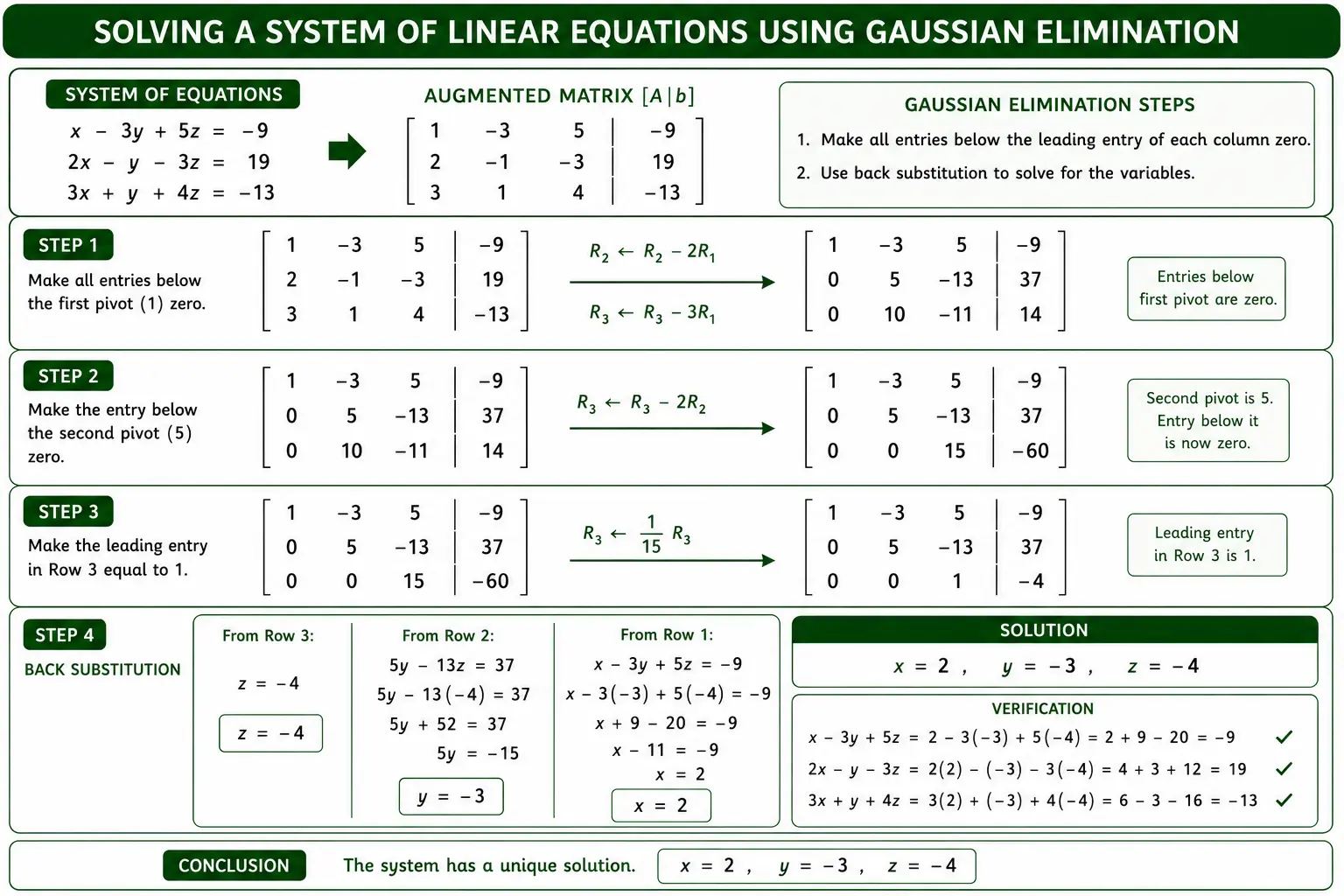
Gaussian Elimination Method is a process of applying Elementary Row Operations to bring the Augmented Matrix into a special form called Row Echelon Form for easy solutions like this for a sample 3×3 matrix.
$$ \left[\begin{array}{ccc|c} 1 & 2 & 3 & 10 \\ 4 & 5 & 6 & 15 \\ 7 & 8 & 9 & 20 \end{array}\right] \Rightarrow \left[\begin{array}{ccc|c} \ast & \ast & \ast & \ast \\ 0 & \ast & \ast & \ast \\ 0 & 0 & 1 & b_3 \end{array}\right] $$
Since matrix multiplication of \([0, 0, 1]\) and \([x_1, x_2, x_3]^T\) results in \(x_3\), we can directly equate it with \(b_3\). Once we solve \(x_3\) we can solve \(x_2\) as well from previous row where there are two unknowns \(x_2\) and \(x_3\) using back substitution. This process continues until all \(x_i\)’s are not solved.
Here is one example.
Gauss-Jordan Elimination Method
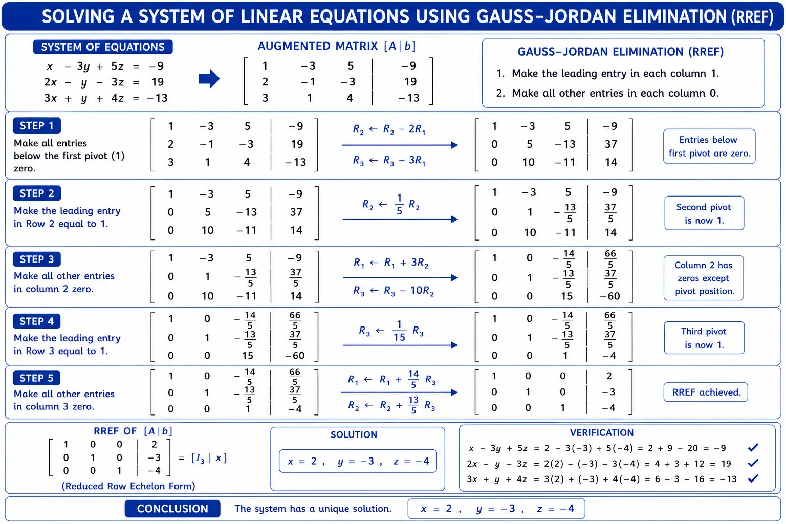
Gauss-Jordan Elimination Method is a process of applying Elementary Row Operations to bring the Augmented Matrix into a strict special form called Reduced Row Echelon Form for direct solutions like this for a sample 3×3 matrix.
$$ \left[\begin{array}{ccc|c} 1 & 2 & 3 & 10 \\ 4 & 5 & 6 & 15 \\ 7 & 8 & 9 & 20 \end{array}\right] \Rightarrow \left[\begin{array}{ccc|c} 1 & 0 & 0 & \ast \\ 0 & 1 & 0 & \ast \\ 0 & 0 & 1 & \ast \end{array}\right] $$
Since it is an identity matrix where all the positions on principle diagonal are populated exactly with 1, we can directly solve for all \(x_i\)’s together without the need of back substitution.
The example below illustrates this.
Solution Through Matrix Inverse
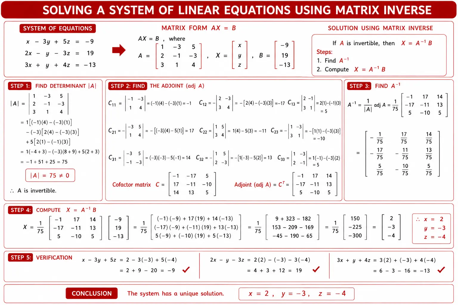
We briefly touched upon this that solution \(X\) can be derived directly from \(A^{-1}b\) as well but matrix inverse for a \(n \times n\) matrix is a costly \(O(n^3)\) process. There are approaches to simplify matrix inverse that we will learn later but the illustration below shows how matrix inverse solve the linear equations.
Column Space
This is one of the four fundamental subspaces of a matrix. Column space specifies the span of the column vectors of the feature matrix \(A\).
Since \(AX\) represents the transformation of \(X\) using \(A\), all the linear combinations possible from the column vectors of \(A\) and its multiplication with \(X\) should remain within the column space of \(A\).
So, if there is some solution to \(AX = b\), then the solution should be part of the column space of \(A\).
In case, if all the columns are not linearly independent, the column space is formed by the span of basis. The dimension of the column space should be same as the rank of the matrix \(A\).
Row Space
Each row of \(A\) represents one equation that acts as a constraint on the solution of linear equations. Row space is defined by the span or linear combinations of the row vectors from \(A\) and dimension of the row space should be same as the rank of the matrix \(A\).
Null Space
If for any input, the matrix \(A\) zero or no output, then that specific input forms the Null space. It is the solution of \(AX = 0\) equation in matrix form.
The transformation \(A\) collapses the vector \(X\) to zero making the transformation irreversible. The trivial solution to \(AX = 0\) is \(X = 0\) but if there is any other form for vector \(X\) for which \(AX = 0\) then the matrix \(A\) is non-invertible and there is no unique solution.
Another way of looking at null space is through uncertainty. If null space contains anything apart from zero vector then we cannot figure out exact \(X\); hence there is no unique solution.
We have started from \(AX = b\). Let’s make \(X\) as \(X + X_\Delta\).
Then
$$ A(X + X_\Delta) = AX + AX_\Delta = b + 0 = b $$
So, we have added additional vectors to original solution \(X\) and still getting same output \(b\) signifying null space contains vectors which can be added without changing the output and producing yet another solution. This again gives us an intuition for redundant feature directions that can be added to the solution vector without affecting the output.
Another important observation arises from the fact that \(AX = 0\). Since dot product between all row vectors and \(X\) are zero, null space is actually orthogonal to row space.
Left Null Space
Another way of determining redundancy or finding out attributes that do not contribute to the pattern recognition process is through Left Null Space. It consists of column vectors \(X^T\) such that \(X^T A = 0^T\). It is same as the null space of \(A^T\).
Since dot products between column vectors of \(A\) and \(X^T\) are all zero, all column vectors are perpendicular i.e. orthogonal to \(X^T\). So, left null space is orthogonal to column space.
Rank-Nullity Theorem
The rank of a matrix is equal to the dimension of the column space or row space of a matrix. For a matrix with \(m \times n\) dimensions where \(m \neq n\), rank is \(minimum(m, n)\).
Rank captures the linearly independent attributes of the feature matrix and the dimension of null space is called Nullity which captures the number of free variables that can take any value without changing the outcome.
So for any feature matrix, the directions that are linearly independent and capture the structure of the feature space, contribute to the rank and the attributes that diminish to zero and don’t add any value, contribute to nullity.
In summary, for a \(m \times n\) matrix \(A\) -
$$ Rank(A) + Nullity(A) = Number\ of\ Unknowns\ n $$