
In the previous blogs we discussed data representation, transformation, the hidden structures of the transforming matrix and how it defines the solution of a system of linear equations. Matrix subspaces control what can be a possible output and identify the data redundancy. The objective of doing all this is to find out solution(s) to a set of linear equations formed by the input observations and expressed in a compact way as \(AX = b\). But what will happen if the solution does not lie within the span of column vectors of the feature space? This possibility inspires us to look at the idea of projection and the closest solution we can get.
Orthogonality
Orthogonality as a direct outcome from the dot product between two different vectors helps the AI/ML system to detect features that have independent directions of variation. So, changes in one feature does not affect another and it stabilizes their learning process.
Orthonormal Set
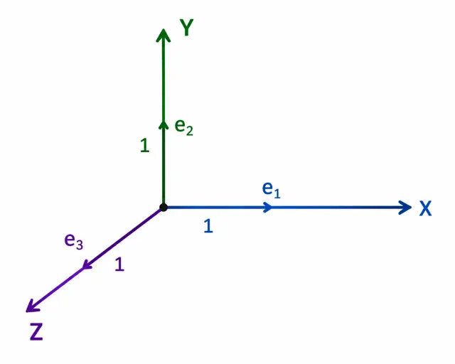
A set of orthogonal/perpendicular set of unit vectors (normalized) of length 1 is called an orthonormal set.
A set of vectors in a finite dimensional vector space is called an orthonormal set if
- They are orthogonal \(\Rightarrow u_i \cdot u_j = 0 \text{ for } i \neq j\)
- They are normalized \(\Rightarrow u_i \cdot u_i = ||u_i||^2 = 1 \text{ for all } i \Rightarrow ||u_i|| = 1 \text{ for all } i\)
Orthonormal Bases
We know from our earlier discussion that Basis of vector space -
- Spans the vector space.
- They are linearly independent.
The basis will be Orthonormal if
- Every basis vector pair is orthogonal.
- Every basis vector is normalized i.e. of length 1.
So, from a feature matrix if we can find out the basis then we will be able to find out the key structural component of that feature space because any vector can be computed using linear combinations of basis vectors and secondly, basis vectors are orthogonal signifying independent directions.
Orthogonality ⇒ Linear Independence but the converse is not True
Orthogonal Matrices
A square matrix \(Q = (q_1, q_2, …, q_n)\) whose columns are orthonormal vectors is called an orthogonal matrix.
An example can be Identity matrix (\(I\)).
Let’s define
$$ Q = \begin{bmatrix} \frac{\sqrt{2}}{2} & -\frac{\sqrt{2}}{2} \\ \frac{\sqrt{2}}{2} & \frac{\sqrt{2}}{2} \end{bmatrix} $$
as an orthogonal matrix. Then
$$ Q^T Q = \begin{bmatrix} \frac{\sqrt{2}}{2} & \frac{\sqrt{2}}{2} \\ -\frac{\sqrt{2}}{2} & \frac{\sqrt{2}}{2} \end{bmatrix} \times \begin{bmatrix} \frac{\sqrt{2}}{2} & -\frac{\sqrt{2}}{2} \\ \frac{\sqrt{2}}{2} & \frac{\sqrt{2}}{2} \end{bmatrix} = \begin{bmatrix} 1 & 0 \\ 0 & 1 \end{bmatrix} = I $$
This implies, \(Q^{-1} = Q^T\)
This is a very important result because we all know matrix inverse is a resource intensive process. So, for any matrix if we can bring it in orthogonal matrix form then we can simply transpose the matrix to get the inverse.
The question now is how do we achieve this conversion. The answer is Gram-Schmidt process which enables this conversion in the same space they originally span using a step by step method.
From Orthogonal Direction to Projection
Our goal is still finding out the vector \(X\) that solves \(AX = b\). But it may happen that the target vector \(b\) does not lie in the column space of \(A\). How do we then get the best possible solution? The approach is called Projection where we try to find out another vector closest to \(b\) but lies within the column space of \(A\).
If the columns of \(A\) are not perpendicular then projection becomes clumsy because of overlapping directions and it becomes difficult to capture individual contribution of each vector; so conversion of matrix \(A(v_1, v_2, …, v_n)\), to a matrix with orthonormal columns \(Q(q_1, q_2, …, q_n)\) provides a clear, perpendicular view of the subspace.
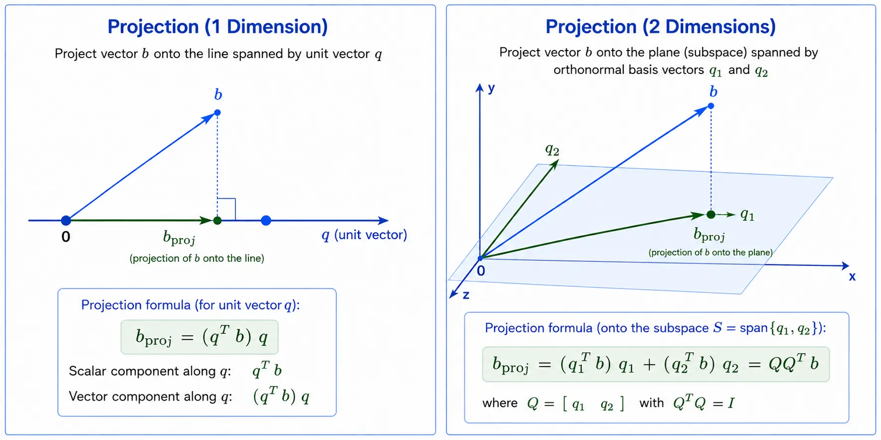
Now if we want to know how much of \(b\) lies along each direction of the orthogonal matrix. We can simply calculate the dot product between \(b\) and \(q_i\) which will be a scalar value.
Multiplying this dot product by \(q_i\) gives us the component of \(b\) along the direction of \(q_i\) and that is the projection of \(b\) on \(q_i\): \((q_i^T b)q_i\).
If we do this for all \(q_i\)’s and sum, we eventually get the projection of \(b\) onto the subspace.
For a single dimension,
$$ b_{proj,i} = (q_i^T b)q_i $$
For all the dimensions, it can be written in matrix form as,
$$ b_{proj} = (q_1^T b)q_1 + (q_2^T b)q_2 + … + (q_n^T b)q_n $$
$$ b_{proj} = (QQ^T)b $$
So, the Projection Matrix \(P\) becomes \(QQ^T\).
One subtle point to note here that \(Q\) is a matrix with orthonormal columns but need not necessarily be a square orthonormal matrix. So, though \(Q^T Q\) is an identity matrix, \(QQ^T\) is a projection matrix rather than an identity matrix.
How Well is The Projection?
The closeness between \(b_{proj}\) and \(b\) determines the quality of the projection. There can be multiple vectors in the subspace \(S\) to project but the one with least distance to \(b\) should be chosen.
The best projection is
$$ b_{proj} = argmin_{z \in S} ||b - z|| $$
The Unexplainable Residual
Since \(b_{proj}\) belongs to the column space of the feature matrix \(A\), \(b_{proj}\) is basically explainable by the features. Since the true observed values is \(b\), there is a difference between them which is captured as residual. Residual is that component that cannot be explained by the attributes.
$$ Residual\ r = b - b_{proj} $$
Direction of Residual
Suppose there is some arbitrary point \(p\) on the subspace and there are two components of the residual \(r\) -
- Along the subspace \(r_{\parallel}\)
- Perpendicular to the subspace \(r_{\perp}\)
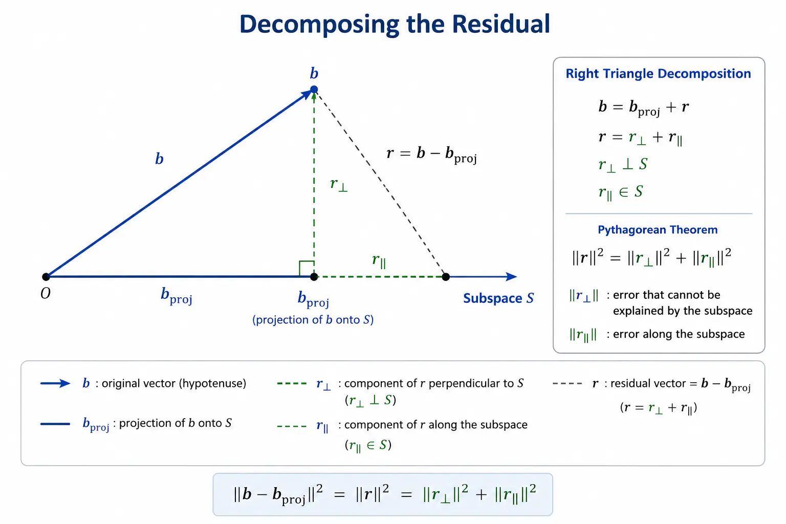
Then total error satisfies the Pythagorean relationship as -
$$ ||b - p||^2 = ||r_{\perp}||^2 + ||r_{\parallel}||^2 $$
If we look at above diagram carefully, we will notice that if there is any component along the subspace, \(r_{\parallel}\) then,
$$ ||b - p||^2 > ||r_{\perp}||^2 $$
So, the shortest possible error occurs when \(r_{\parallel} = 0\) signifying residual \(r\) is perpendicular to the subspace \(S\).
As a consequence, dot product between any column vector \(q_i\) and residual \(r\) is Zero and for the entire matrix we can write
$$ Q^T r = 0 $$
confirming residual has zero component along every direction of the subspace.
Orthogonal Complements
Since \(b = b_{proj} + r\) where \(b_{proj}\) belongs to subspace \(S\) and explainable by the column vectors of the feature matrix. Residual \(r\) is what the model cannot explain and it is orthogonal to the subspace.
Theoretically there exists a set of vectors \(S^{\perp}\) perpendicular to all the vectors of subspace \(S\) and residual \(r \in S^{\perp}\).
This component \(S^{\perp}\) is called Orthogonal Complement representing directions invisible to feature space.
Since the subspace \(S\) is formed by the column space of feature matrix \(A\), we can say that residual lies in the orthogonal complement of column space of \(A\).
Matrix Factorization
There are approaches to decompose the matrix into simpler components as an efficient solution strategy for the system of linear equations. We will discuss two of them here.
QR Decomposition
For a matrix \(A\), apply Gram-Schmidt method to get a matrix with Orthonormal components \(Q\) and another Upper triangular matrix \(R\) containing the coefficients required to reconstruct \(A\). This is very useful for projection and gives numerically stable orthonormal representations of the column space.
\(A = QR\)
Example:
$$ \begin{bmatrix} 1 & -1 \\ 1 & 4 \end{bmatrix} = \begin{bmatrix} \frac{1}{\sqrt{2}} & -\frac{1}{\sqrt{2}} \\ \frac{1}{\sqrt{2}} & \frac{1}{\sqrt{2}} \end{bmatrix} \times \begin{bmatrix} \sqrt{2} & 3\sqrt{2} \\ 0 & 5\sqrt{2} \end{bmatrix} $$
LU Decomposition
It breaks the matrix \(A\) into two components - Lower triangular matrix (\(L\)) and Upper triangular matrix (\(U\)) so that the Gaussian elimination method can become faster.
\(A = LU\)
Example:
$$ \begin{bmatrix} 2 & 1 \\ 4 & 3 \end{bmatrix} = \begin{bmatrix} 1 & 0 \\ 2 & 1 \end{bmatrix} \times \begin{bmatrix} 2 & 1 \\ 0 & 1 \end{bmatrix} $$
We can visually inspect different subspaces of any matrix here.