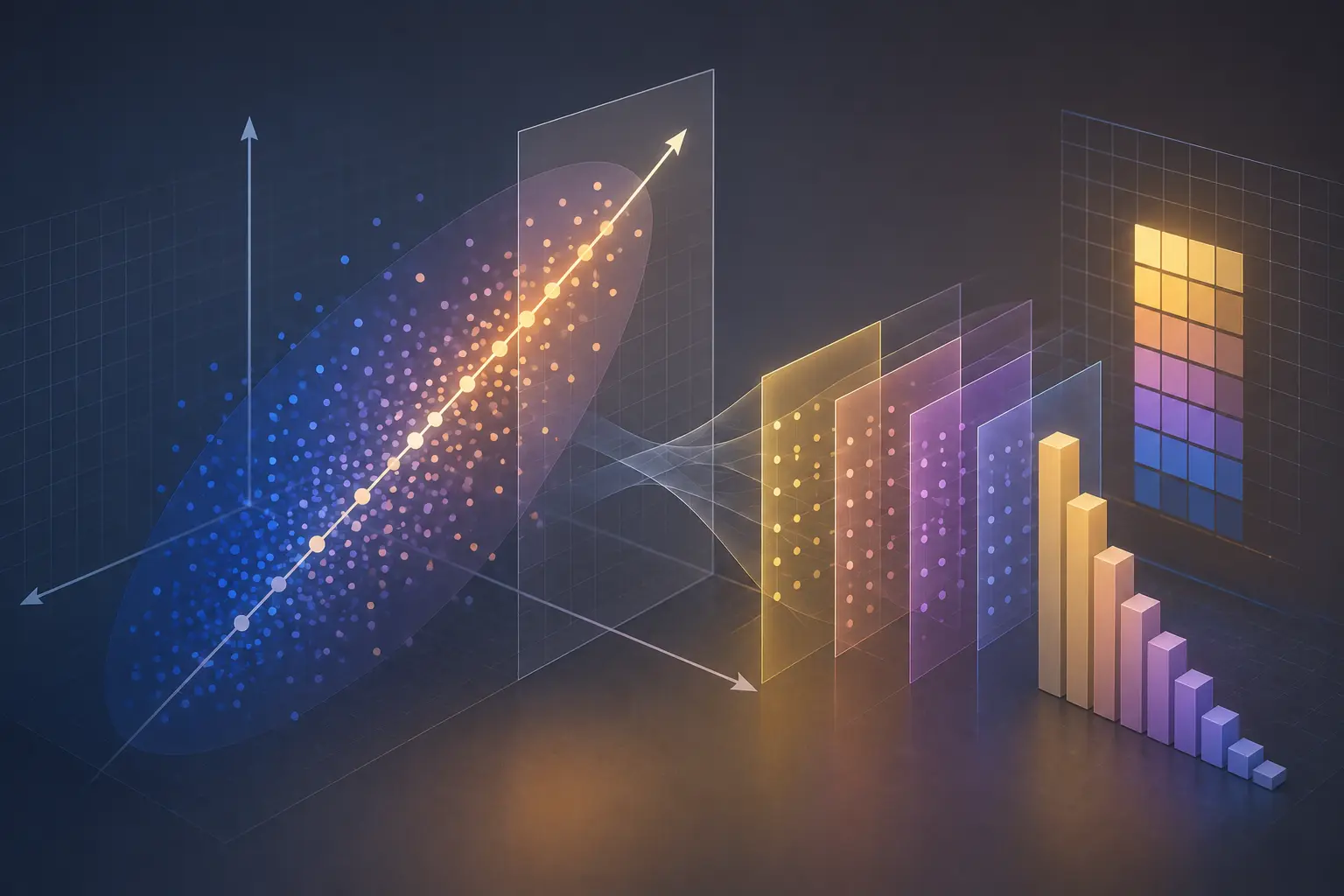
What did we learn till now? We understood how data is represented as vectors, why data transformation is a matrix multiplication, how to find out key attributes and remove data redundancy, different forms of solutions to the systems of linear equations, the role of four fundamental vector subspaces and finally how projection helps find best possible approximation. But is there a way of knowing what are the directions along which the data has maximum variability? If so, then we can use only those dimensions discarding others, simplifying the representation of the system. Similarly, were we able to identify any vector that remains directionally invariant during data transformation and provide stability? In this blog we will try to answer these two questions and uncover the math behind them.
Directional Invariance
When a matrix transforms an entire space, usually the direction and magnitude of all the vectors get changed. But during observation it is found out that there are some vectors that don’t change the direction, rather they either stretch or shrink. These vectors act like axes of the space and capture the maximum variability or spread of the data.
These vectors are called Eigenvectors and the magnitude of stretch/shrink is called Eigenvalue. Eigenvectors appear to be the natural direction of the transformation where the data itself dictates its own axis which can be completely different from the regular \(x\), \(y\) or \(z\)-axes.
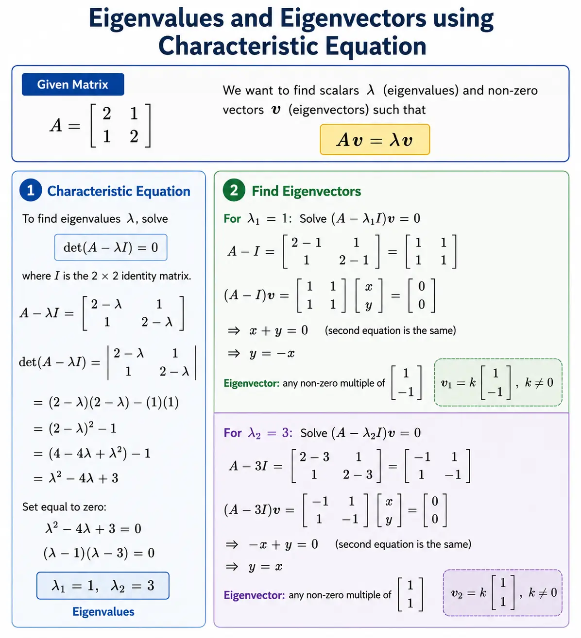
Any matrix \(A\) can have multiple Eigenvalue-Eigenvector pairs. For any pair, if the Eigenvalue and Eigenvector are \(\lambda\) and \(v\) respectively, then
$$ Av = \lambda v $$
$$ \Rightarrow (A - \lambda I)v = 0 $$
For a non-zero solution to exist, \((A - \lambda I)\) must be Singular.
$$ \Rightarrow determinant(A - \lambda I) = 0 $$
This is called the Characteristic Equation.
Let’s check one example to understand the concept.
We mentioned that Eigenvectors remain directionally invariant after transformation which is evident in the below geometric depiction.
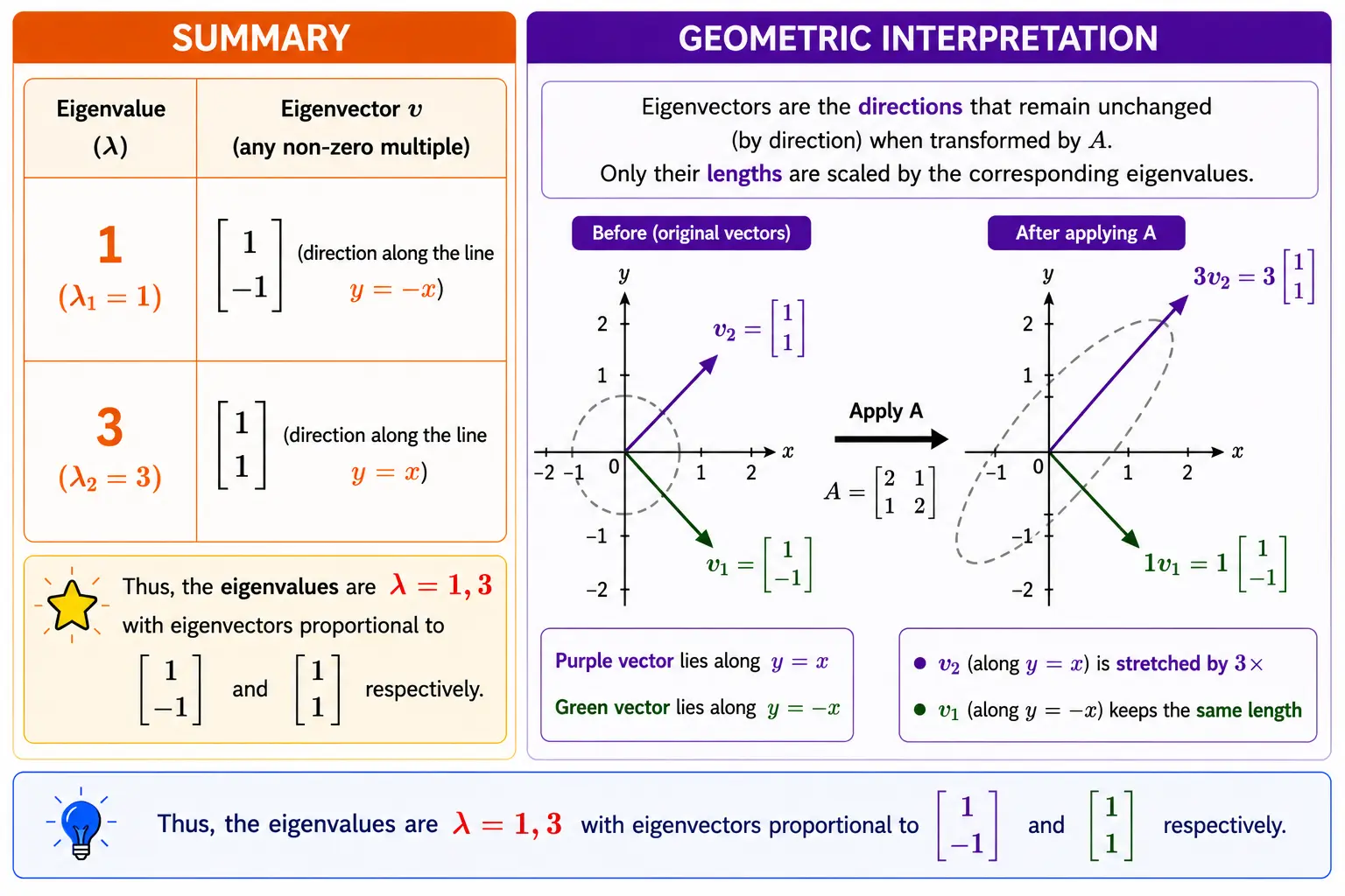
One important outcome is when \(\lambda = 0\), \(Av = 0\) too signifying \(v\) belongs to the Null Space of \(A\).
Alternate Co-ordinate System
In the \(x, y\) co-ordinate the transformation is defined by matrix
$$ A = \begin{bmatrix} 2 & 1 \\ 1 & 2 \end{bmatrix} $$
let’s create a matrix \(V\) whose columns are Eigenvectors of \(A\) (keeping the Eigenvector of largest Eigenvalue as the first column).
$$ V = \begin{bmatrix} 1 & 1 \\ 1 & -1 \end{bmatrix} $$
The effect of applying transformation \(A\) on \(V\) is:
$$ A \times V = \begin{bmatrix} 2 & 1 \\ 1 & 2 \end{bmatrix} \times \begin{bmatrix} 1 & 1 \\ 1 & -1 \end{bmatrix} $$
$$ \Rightarrow A \times V = \begin{bmatrix} 3 & 1 \\ 3 & -1 \end{bmatrix} $$
$$ \Rightarrow \begin{bmatrix} 1 & 1 \\ 1 & -1 \end{bmatrix} \times \begin{bmatrix} 3 & 0 \\ 0 & 1 \end{bmatrix} = V \times \Lambda $$
$$ \Rightarrow AV = V\Lambda $$
$$ \Rightarrow A = V\Lambda V^{-1} $$
So, when any vector is described using the Eigenvector directions as the new co-ordinate system, the transformation simply becomes
$$ \Lambda = \begin{bmatrix} 3 & 0 \\ 0 & 1 \end{bmatrix} $$
Diagonalization
The transformation matrix in the new co-ordinate system is a Diagonal matrix where the largest Eigenvalue is placed in the first column and second largest one in the second column. Since it is a diagonal matrix, only one element in each column will be non-zero which makes column vectors as independent. So, the diagonal matrix of Eigenvalue provides the directions of independent transformations.
It also makes computations simpler.
Since,
$$ A = V\Lambda V^{-1} $$
$$ A^k = V\Lambda^k V^{-1} $$
and for this 2x2 matrix
$$ \Lambda^k = \begin{bmatrix} \lambda_1^k & 0 \\ 0 & \lambda_2^k \end{bmatrix} $$
Diagonalization is also called Eigendecomposition because it decomposes a transformation matrix into Eigenvector directions and corresponding Eigenvalues.
Spectral Decomposition
For symmetric matrices, if the Eigenvectors are chosen to be Orthonormal, then transformation matrix \(A\) can be written as
$$ A = Q\Lambda Q^T $$
where \(Q\) is the matrix of orthonormal Eigenvectors. This is called Spectral Decomposition.
Which Directions Matter Most?
Each Eigenvalue tells us the magnitude of the transformation along the corresponding Eigenvector. The magnitude acts as a measure of strength of transformation. So, in our example above the magnitude is higher in the direction of Eigenvector \([1, 1]^T\) and this direction becomes a dominating axis.
So, if we have \(N\) number of Eigenvalues, we can sort them into descending order and get an idea of relative dominance of the corresponding Eigenvector in terms of how strongly the transformation acts along those directions.
Singular Value Decomposition
Eigenvalues determine how much stretch is possible for directionally invariant vectors and the calculation demands the matrix to be a square matrix. But if the matrix is not square and/or we want to find out the maximum stretch possible in any direction then the approach is slightly different and is called Singular Value Decomposition (SVD).
Singular Values capture the stretch in any direction and SVD is basically an approach of finding out orthogonal directions whose magnitude of stretch is controlled by singular values. The orthogonal directions are ordered on the basis of descending singular values.
The singular values are represented as \(\sigma_i\) such that
$$ \sigma_1 \geq \sigma_2 \geq \sigma_3 \geq … \geq 0 $$
For any matrix \(A\), the normalized (unit length) Eigenvectors \(v_i\)’s are calculated from \(A^T A\) which captures all the directional pulling, stretching energy of \(A\).
If we apply the transformation \(A\) which is a \(m \times n\) matrix on any \(v_i\) we get -
$$ Av_i = \sigma_i u_i $$
where \(u_i\) specifies post transformation direction for \(v_i\).
It can be written in matrix form as -
$$ AV = [\sigma_1 u_1, \sigma_2 u_2, …, \sigma_n u_n] $$
where \(V\) contains all \(v_i\)’s which are all Orthonormal.
$$ \Rightarrow AV = [u_1, u_2, …, u_m] \begin{bmatrix} \sigma_1 & & \\ & \ddots & \\ & & \sigma_n \end{bmatrix} $$
$$ \Rightarrow AV = U\Sigma $$
$$ \Rightarrow AVV^T = U\Sigma V^T $$
$$ \Rightarrow A = U\Sigma V^T $$
Since Eigenvalues are calculated from \(A^T A\), the effect of stretch is realized twice making the total stretch factor as \(\sigma \times \sigma = \sigma^2\). So, each Eigenvalue \(\lambda = \sigma^2\) and we can say
\(Singular\ Value = \sqrt{Eigenvalue}\)
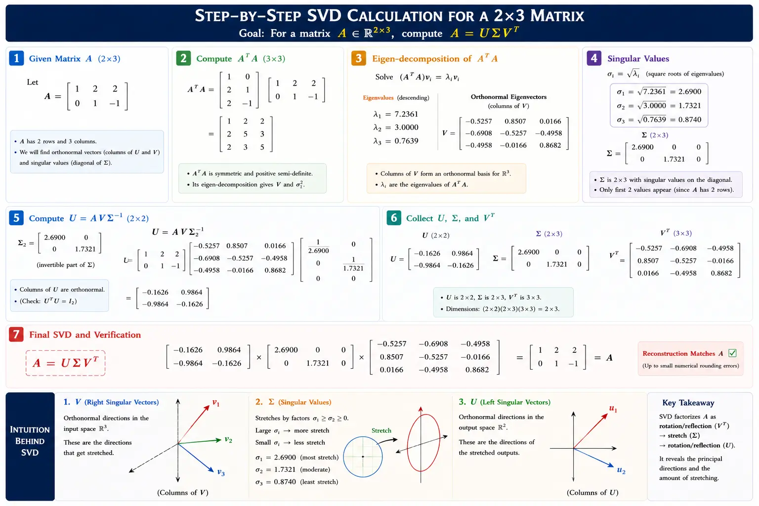
The numerical example for SVD calculation is shown below.
Low Rank Approximation
The rank of a matrix is equal to the number of non-zero singular values it has and singular values are the building blocks of SVD factorization.
Let’s think of an image of dimension \(4096 \times 4096\) and we want to compress it to \(1024 \times 1024\) pixels. The obvious question is how do we select 1024 pixels from 4096? We definitely want to select those 1024 pixels that contain maximum structural information.
The approach here is to have the singular values calculated and identify \(top-k\) singular values that captures maximum information, then approximate \(A\) with \(A_k\) and apply SVD -
$$ A \approx A_k = \sum_{i=1}^{k} \sigma_i u_i v_i^T $$
Since we considered only \(k\) singular values, the rank of \(A_k\) is \(k\) which is smaller than the rank of original matrix \(A\). This is called Low Rank Approximation that acts as a dimensionality reduction technique.
Here we can see different forms of matrix factorization.
This six-part series builds the mathematical foundations for AI/ML focusing on geometric representations of data and its linear transformations. It culminates how linear algebra unearths structure in the data. Next, we will explore Calculus to understand the learning process of AI/ML algorithms.