In the previous two parts we have dealt with Probability and fundamentals of Random Variables. We have understood how random variables abstract the physical events and map them into real numbers with associated probability. We have mainly discussed individual random variables each of which represents a particular event. But in reality, physical events interact with each other and we need to explore how they behave together. In this article, we will go through the different properties of co-occurrence of random variables.
The Multiverse of Co-occurring Events
As mentioned in the introductory note, when events occur simultaneously affecting each other then their combined probability is captured mathematically through Joint Probability Distributions. It is represented as the following.
$$ P_{XY}(X,Y)=P(X=x,Y=y) \qquad \text{for discrete case} $$
$$ f_{XY}((X,Y)\in A)=\int_{}\int_{A}f_{XY}(X,Y)dydx \qquad \text{for continuous case} $$
Since it is a probability distribution, the sum is 1.
$$ \sum_x \sum_y P_{XY}(X,Y)=1 \qquad \text{for discrete case} $$
$$ \int_{-\infty}^{\infty}\int_{-\infty}^{\infty}f_{XY}(X,Y)dxdy=1 \qquad \text{for continuous case} $$
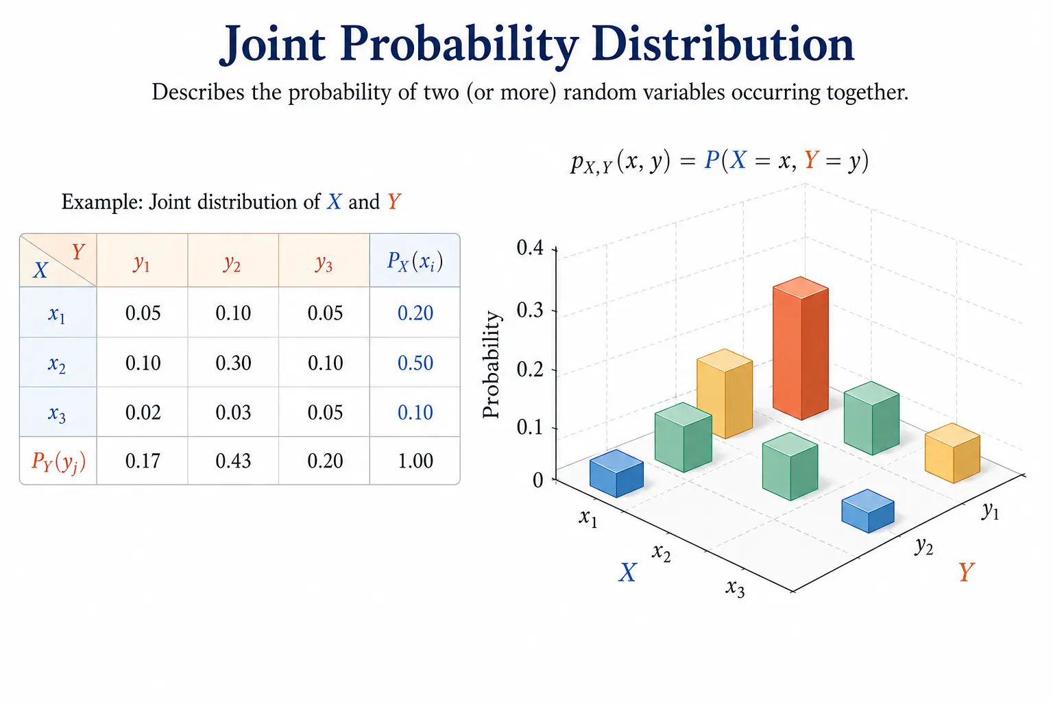
Joint CDF can be calculated as
$$ F_{XY}(a,b)=P(X\le a,Y\le b) $$
Isolating a Single Signal
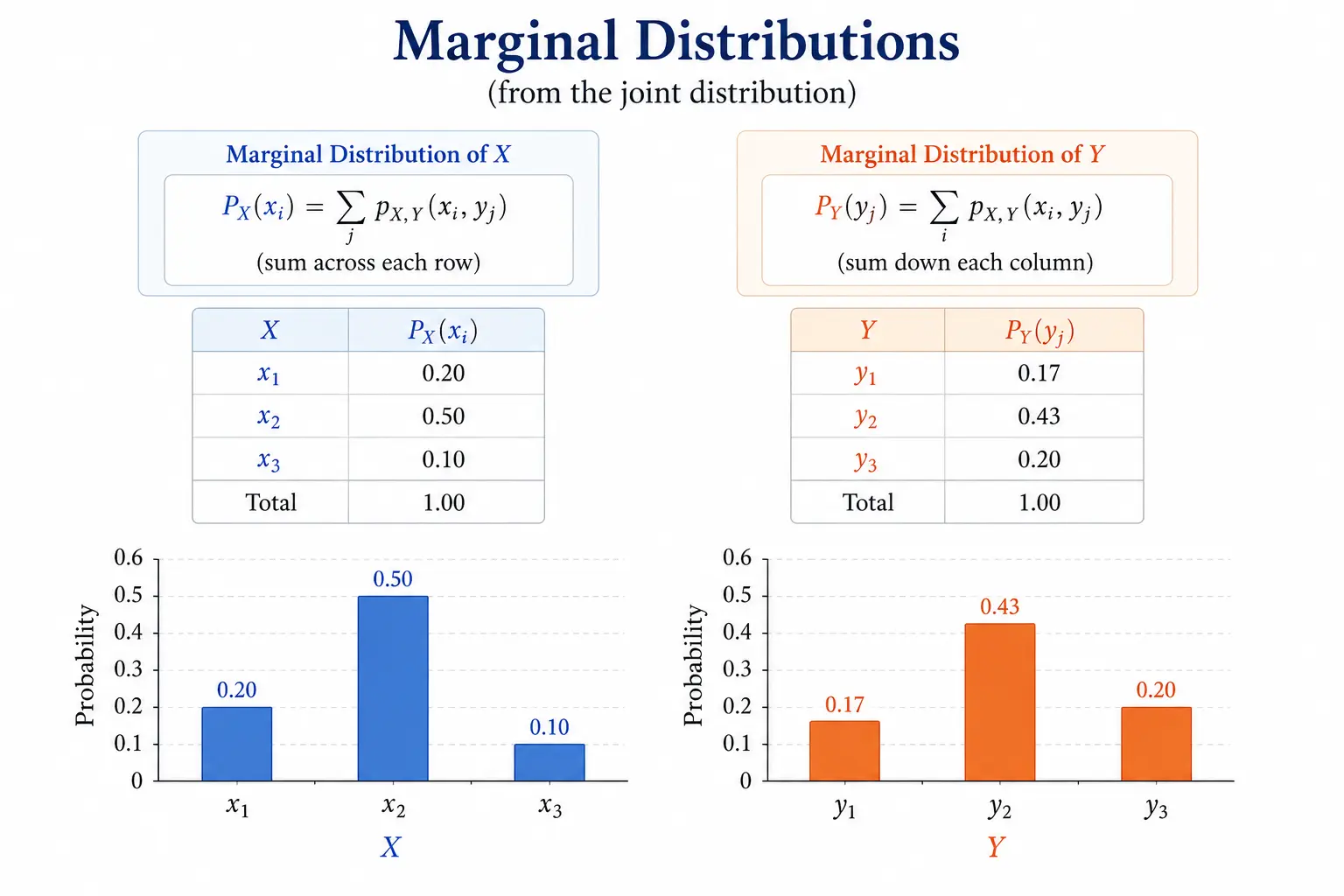
From a joint distribution, if it is required to isolate the distribution of a single event represented through its own random variable, then it is done by taking the sum/integrate over all the values of the other variable for discrete and continuous cases respectively. This is called Marginal Probability Distribution of that isolated variable.
$$ P(X)=\sum_{Y=y}P_{XY}(X,Y) $$
$$ P(Y)=\sum_{X=x}P_{XY}(X,Y) \qquad \text{for discrete case} $$
$$ P(X)=\int_{-\infty}^{\infty}f_{XY}(X,Y)dy $$
$$ P(Y)=\int_{-\infty}^{\infty}f_{XY}(X,Y)dx \qquad \text{for continuous case} $$
Updating Expectations with Context
Similar to conditional probability we can derive Conditional Expectation where the expected value gets changed due to the occurrence of another event. It is the expectation of Event \(X\) occurring under the assumption that Event \(A\) is already confirmed or occurred.
$$ E(X|A)=\sum_x x \cdot P(X=x|A) \qquad \text{for discrete RV} $$
$$ E(X|A)=\int_{-\infty}^{\infty}x\cdot f_{X|A}(x|A)dx \qquad \text{for continuous RV} $$
The Tower of Averages
The expectation of a random variable \(X\) can be derived from calculation of the expectation of the conditional expectation of \(X\) given another variable \(Y\). This is called the Law of Iterated Expectations or Tower Property.
Let, \(X\) and \(Y\) are discrete random variables.
$$ E(E(X\mid Y)) = \sum_y E(X\mid Y=y)\cdot P(Y=y) $$
$$ E(E(X\mid Y)) = \sum_y\left(\sum_x x\cdot P(X=x\mid Y=y)\right)P(Y=y) $$
$$ E(E(X\mid Y)) = \sum_x\sum_y x\cdot P(X=X\mid Y=y)\cdot P(Y=y) $$
$$ E(E(X\mid Y)) = \sum_x x \sum_y P(X=X\mid Y=y)\cdot P(Y=y) $$
$$ E(E(X\mid Y)) = \sum_x x \sum_y P(X=x,Y=y) \qquad \text{(from conditional to joint distribution)} $$
$$ E(E(X\mid Y)) = \sum_x x\cdot P(X) \qquad \text{(from joint to marginal distribution)} $$
$$ \qquad \text{So, } E(E(X\mid Y)) = E(X) $$
Similar derivation can be computed for continuous random variables by replacing \(sum\) with \(integration\). The advantage of this property is to break down the complex calculation into hierarchical stages.
Measuring Variability with Context
The variance can also be updated once it is known that some event \(A\) is known or has already happened. This quantifies the Conditional Variance.
$$ Var(X|A)=E(X^2|A)-E(X|A)^2 $$
The Law of Total Variance (Eve’s Law) ties variance and conditionals together.
$$ Var(X)=Expectation(Var(X|A))+Var(Expectation(X|A)) $$
The Ripple of Accumulated Uncertainty
For a multi-dimensional dataset if we want to measure the variability or total spread of a combined set of variables then the Sum of Variance comes into effect. Mathematically it can be represented as below.
For the 2-variable case,
$$ Var(X+Y) = Var(X)+Var(Y)+2\cdot Cov(X,Y) $$
For the general case,
$$ Var\left(\sum_{i=1}^{n}X_i\right) = \sum_{i=1}^{n}Var(X_i) + 2\sum_{i,j:i\neq j}Cov(X_i,X_j) $$
Measuring the Shared Variability
Joint probability distribution was the first step where concepts of multiple variables occurring simultaneously arose. Covariance is one step ahead in the realm of co-occurrence where the magnitude and direction of the linear relationship among multiple random variables is measured.
$$ Cov(X,Y) = E[(X-E(X))(Y-E(Y))] $$
$$ Cov(X,Y) = E[XY-XE(Y)-E(X)Y+E(X)E(Y)] $$
$$ Cov(X,Y) = E(XY)-E(X)E(Y)-E(X)E(Y)+E(E(X)E(Y)) $$
$$ Cov(X,Y) = E(XY)-E(X)E(Y) $$
The covariance of a variable with itself is simply the variance.
$$ Cov(X,X)=Var(X) $$
For more than 2 variables, we need a Covariance Matrix.
For a 3 variable scenario, the covariance matrix is:
$$ \begin{bmatrix} Var(X) & Cov(X,Y) & Cov(X,Z) \\ Cov(Y,X) & Var(Y) & Cov(Y,Z) \\ Cov(Z,X) & Cov(Z,Y) & Var(Z) \end{bmatrix} $$
Correlation, on the other hand, quantifies both the strength and direction of the relationship in a unitless fashion using Correlation Coefficient \(ρ\).
$$ \rho(X,Y) = \frac{Cov(X,Y)}{Std.Dev(X)\cdot Std.Dev(Y)} $$
or
$$ \rho(X,Y) = \frac{Cov(X,Y)}{\sigma_X\cdot \sigma_Y} $$
$$ -1 \le \rho \le 1 $$
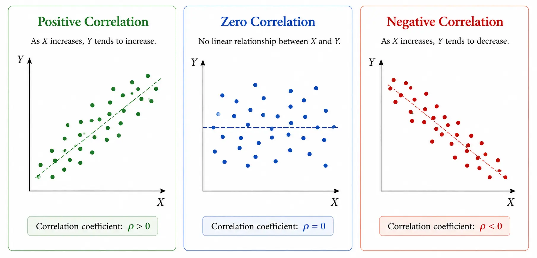
The range of \(ρ\) is between -1 and 1. When correlation is positive then both the variables move in the same direction; when it is negative, both the variables move in the opposite direction and when it is 0, variables are uncorrelated.
There are mainly three ways of defining correlation coefficients - the above approach is called Pearson’s correlation coefficient when the underlying data is continuous, normal and the relationship is linear. The second one is termed as Spearman’s rank correlation coefficient when the underlying data is not normal and it can be continuous, ordinal or interval. The third one is called Kendall’s rank correlation coefficient which is used to measure the similarity of ordering between two measured quantities without the normality and linearity assumptions. Kendall’s rank correlation coefficient ranks the data points in two quantities and for each pair, it tries to find out the agreement by counting the number of concordant (ranks change in the same direction) and discordant pairs (ranks change in the opposite direction).
Understanding Standalone Variables
If knowing some information of one random variable does not alter the understanding of another random variable then it can be said that they are Independent of each other.
For independent random variables correlation coefficient \(ρ\) is 0 but the converse that when \(ρ = 0\) does not necessarily mean that random variables are independent.
So, for sum of independent random variables, the covariance part vanishes.
$$ Var\left(\sum_{i=1}^{n}X_i\right) = \sum_{i=1}^{n}Var(X_i) $$