
From the fundamentals of probability and random variables, we have understood how random variables interact with each other in reality. In this article, we will discuss how samples drawn from underlying distribution help us infer its statistical properties. We will also explore how distributions converge and how we can make assumptions about the population and find evidence for or against them.
The Certainty of Scale
As in Statistics, Law of Large Number (LLN) is a theorem that says if we perform the same experiment a large number of times then the average of the outcomes of the experiments should be close to the true mean. The LLN is important because it guarantees stable long-term results for the averages of some random events (RV) and that is the reason why a casino will always make money in the long run even after losing money in a few instances.
Mathematically, it says that if the same experiment is performed \(n\) (\(n\) is very large) times as independent and identical (i.i.d.) experiments then the numerical average of the outcomes will be very close to the true mean \(\mu\) in probability (Weak) and almost surely (Strong).
Let \(X_1,X_2,\ldots,X_n\) be i.i.d. random variables with same mean \(\mu=E(X_i)\) and variance \(\sigma^2=Var(X_i)\).
Then the Law of Large Numbers says,
$$ \text{Sample average }\bar{X}_n=\frac{1}{n}\sum_{i=1}^{n}X_i\rightarrow\mu\quad\text{as }n\rightarrow\infty $$
Since any linear combination of normal random variables is also normal, in the below example the true mean of data variable is \(5\times0+10=10\). We will see when \(n\) increases from 10 to 100000, the numerical average becomes closer to the true mean 10.
import numpy as np

np.random.seed(1)

data = 5 * np.random.randn(10) + 10
print("Average when n=10 is :", np.mean(data))

data = 5 * np.random.randn(1000) + 10
print("Average when n=1000 is :", np.mean(data))

data = 5 * np.random.randn(10000) + 10
print("Average when n=10000 is :", np.mean(data))

data = 5 * np.random.randn(100000) + 10
print("Average when n=100000 is:", np.mean(data))
The output shows
Average when n=10 is : 9.5142955459695
Average when n=1000 is : 10.184099506736104
Average when n=10000 is : 10.039233155010294
Average when n=100000 is: 10.013670784412874
The Universal Bell Curve
The importance of Gaussian distribution comes from Central Limit Theorem (CLT) which states that under some conditions, the average of many observations of a random variable with finite mean and variance is itself a random variable whose distribution converges to a normal distribution \(N\) as the number of samples increases even if the original variables themselves are not normally distributed.
Let \(X_1,X_2,\ldots,X_n\) be i.i.d. random variables with same mean \(\mu=E(X_i)\) and variance \(\sigma^2=Var(X_i)\).
Mean of sample average,
$$ E(\bar{X}_n)=\frac{n\mu}{n}=\mu $$
$$ Var(\bar{X}_n)=\frac{n\sigma^2}{n^2}=\frac{\sigma^2}{n} $$
Then Central Limit Theorem says,
$$ \bar{X}_n \rightarrow N\left(\mu,\frac{\sigma^2}{n}\right)\quad\text{as }n\rightarrow\infty $$
$$ \frac{\bar{X}_n-\mu}{\sigma/\sqrt{n}} \rightarrow N(0,1) \quad\text{as }n\rightarrow\infty $$
Equivalently,
$$ \sqrt{n}\left(\bar{X}_n-\mu\right) \rightarrow N(0,\sigma^2) \quad\text{as }n\rightarrow\infty $$
# Generate a Sample of Dice Rolls
import numpy as np
import matplotlib.pyplot as plt

np.random.seed(1)

T_n = []
mu = (1 + 2 + 3 + 4 + 5 + 6) / 6
n = 1000

for i in range(n):
    data = np.random.randint(low=1, high=7, size=1000)   # Returns discrete uniform integers
    X_n = np.sum(data) / 1000      # Sample average
    X_c = X_n - mu                 # Subtract true mean μ
    X_f = X_c * np.sqrt(n)         # Multiply by √n
    T_n.append(X_f)

fig = plt.figure(figsize=(20, 10))
plt.hist(T_n, bins=100)
plt.title(
    "Histogram of Sample Means from Dice Roll Simulations",
    fontsize=16
)
plt.xticks(np.arange(-5, 6, 1))
plt.show()
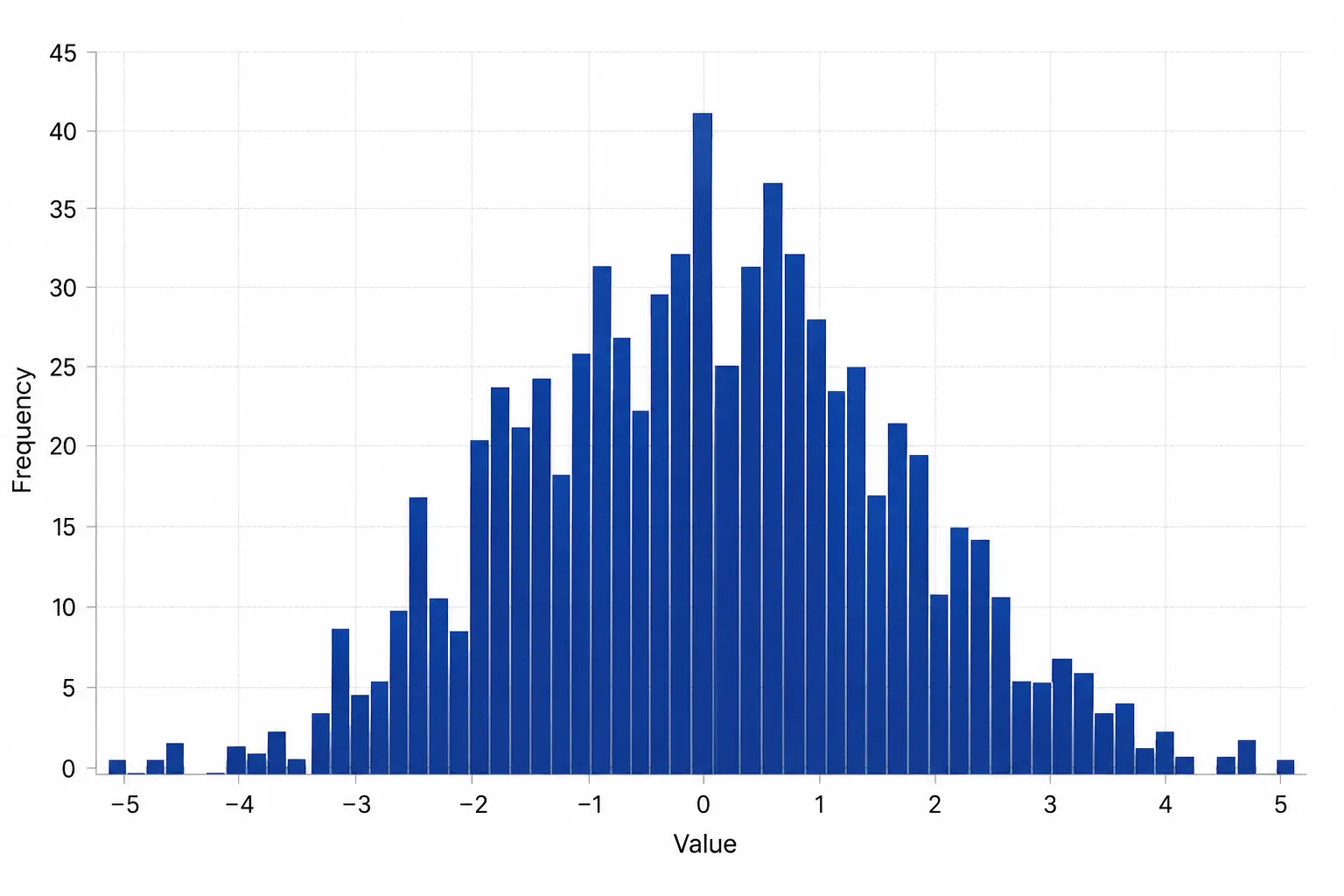
If we plot the histogram of centered sample average after subtracting the true mean and multiplying by \(\sqrt{n}\), we can pictorially conclude that the distribution is Gaussian and the mean is 0.
Decoding the Hidden Truth
Using the observations coming out of a random distribution, we need to infer what kind of distribution it is and what is the parameter that explains the properties of that distribution. It forms the basics of Parameter Estimation, which is the first step of statistical inference.
Defining the Boundary Lines
The advantage of the Central Limit Theorem (CLT) is that for a large number of observations any distribution converges to the Standard Normal Distribution.
$$ \frac{\bar{X}_n-\mu}{\sigma/\sqrt{n}} \rightarrow N(0,1) \quad\text{as }n\rightarrow\infty $$
The left-hand side of the above equation is called the Test Statistic of an experiment. If we can calculate the Test Statistic (Z-score), we can definitely calculate the probability of this Test Statistic being larger than a cut-off value. Conversely, if we know the probability (p-value), we can calculate the cut-off value because the probabilities corresponding to different cut-off values under the Standard Normal Distribution are readily available in the Z-score table (Standard Normal Table).
When estimating a parameter of a population from a sample, a single numerical estimate is generally insufficient because it does not indicate the uncertainty associated with the estimate. Therefore, we estimate an interval within which the true parameter is expected to lie with a specified probability. This interval is called the Confidence Interval.
For a fixed \( \alpha \in (0,1) \), if \(q_{\alpha/2}\) is the \((1-\alpha/2)\)-quantile of the Standard Normal Distribution \(N(0,1)\), then with probability \((1-\alpha)\) (if \(n\) is sufficiently large, i.e., asymptotically), the confidence interval of the estimator becomes
$$\left[\bar{X}_n-q_{\alpha/2}\frac{\sigma}{\sqrt{n}},\bar{X}_n+q_{\alpha/2}\frac{\sigma}{\sqrt{n}}\right]$$
# Confidence Interval
from scipy.stats import norm
import numpy as np

np.random.seed(1)

data = 5 * np.random.randn(100) + 50
q_a_2 = norm.ppf(0.90)

low = np.mean(data) - (q_a_2 * np.std(data)) / np.sqrt(len(data))
high = np.mean(data) + (q_a_2 * np.std(data)) / np.sqrt(len(data))

print("90 percent Confidence Interval is: %.3f, %.3f" % (low, high))
Output:
90 percent Confidence Interval is: 49.736, 50.870
The true mean of the random distribution is 50, but the 90% confidence interval lies between 49.736 and 50.870.
The Calculus of Proof
Hypothesis Testing is a mathematical framework to evaluate claims or beliefs about a population using drawn samples from it and calculating an appropriate Test Statistic around it.
Suppose we have a coin to toss and we assume the coin to be fair, i.e., the probability of obtaining a head is 0.5. This assumption forms the baseline hypothesis of the experiment and is called the Null Hypothesis \(H_0\).
The alternative assumption is that the coin is unfair, which is called the Alternative Hypothesis \(H_1\).
We toss the coin 200 times and obtain 170 heads.
The test statistic becomes
$$ \frac{\sqrt{200}\left(\frac{170}{200}-0.5\right)} {\sqrt{0.5\times0.5}} = 9.89 $$
The value 9.89 is larger than 1.645, which is the 95% quantile (assuming \(\alpha=0.05\)) of the Standard Normal Distribution.
Therefore, we reject the Null Hypothesis and conclude that the coin is unfair.
Type I error of a hypothesis test occurs when the Null Hypothesis \(H_0\) is rejected even though it is actually true (False Positive), whereas Type II error occurs when the Null Hypothesis \(H_0\) is not rejected even though the Alternative Hypothesis \(H_1\) is true (False Negative).
Special Distributions
These types of distributions need to be understood because of their significance.
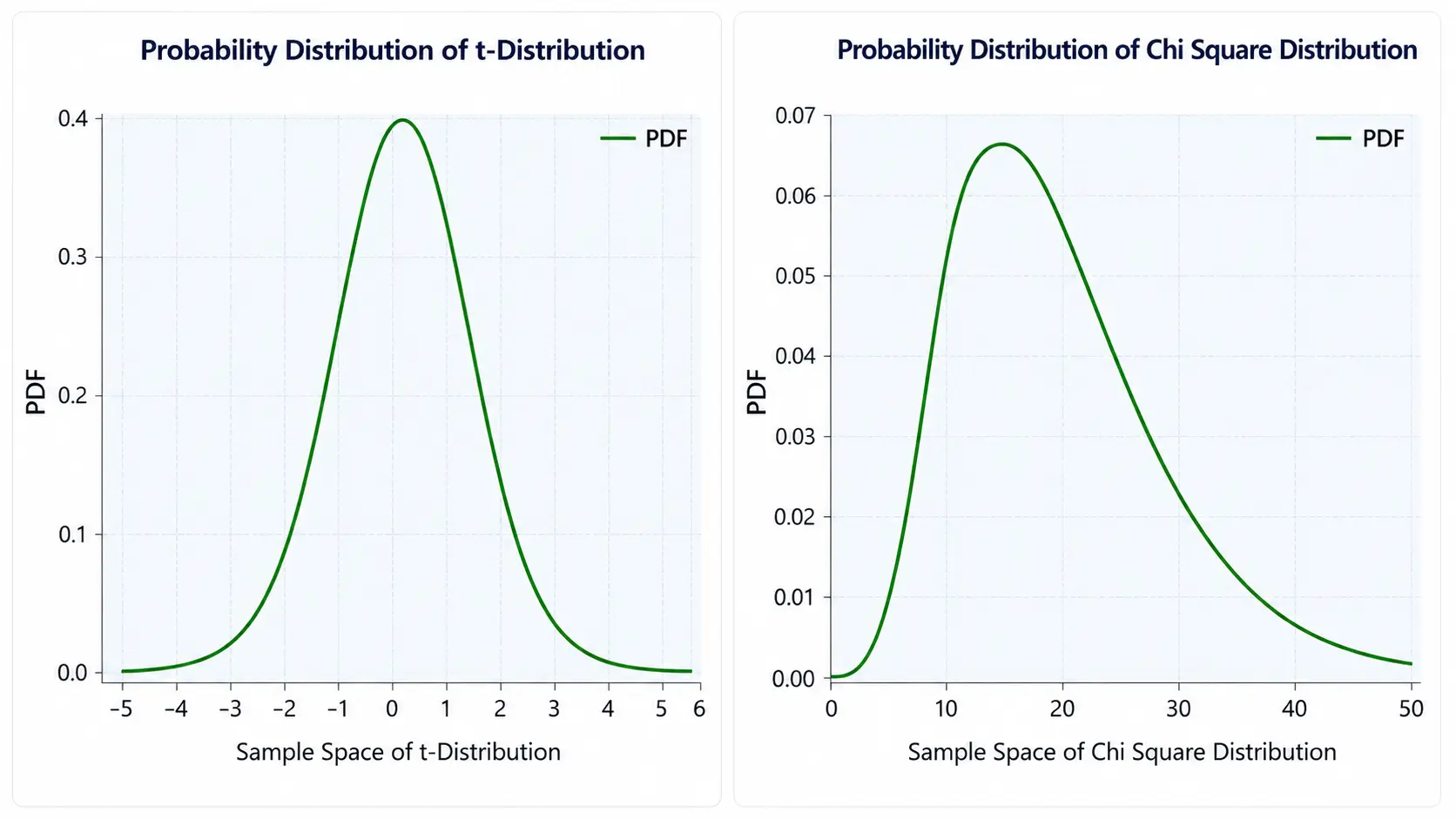
Student’s t-Distribution: The assumption to apply the Central Limit Theorem is that the sample size is large. If it is small (< 30), then the distribution of the random variables follows a Student’s t-distribution instead of the Gaussian distribution.
Chi Square Distribution: The Chi-Square distribution with \(d\) degrees of freedom (number of independent variables) is the distribution of the sum of \(d\) independent standard normal random variables. Therefore, its possible values are always positive. It is used in the Goodness-of-Fit test of a distribution.
Parametric Hypothesis Tests
When a distribution has some parameter, we can create a test statistic using that parameter and leverage it to make assumptions about the underlying distribution and validate them. Here are some of the prominent Parametric Hypothesis Tests that we will discuss.
Student’s t-Test
The Student’s t-test is a statistical hypothesis test where the test statistic follows the t-distribution under the Null Hypothesis. We can think of a case where we want to see if the average height of Indians is statistically different from that of Germans. Since the heights of two different countries follow a normal distribution as per the Central Limit Theorem and they are independent of each other, we can apply the Student’s t-test.
# Student's t-Test
from scipy.stats import ttest_ind
import numpy as np

np.random.seed(1)
# np.random.randn generates Standard Normal data

data1 = 20 * np.random.randn(200) + 50      # mean = 50, standard deviation = 20
data2 = 10 * np.random.randn(200) + 51      # mean = 51, standard deviation = 10

stat, p = ttest_ind(data1, data2)
print("Test Statistic = %.3f, p = %.3f" % (stat, p))
alpha = 0.05      # Our desired confidence interval is 0.95

if p > alpha:
    print("Same distributions (fail to reject H0)")
else:
    print("Different distributions (reject H0)")
It generates the following output.
Test Statistic = 0.799, p = 0.425
Same distributions (fail to reject H0)
Paired Student’s t-Test
Say we measure the blood pressure of a few individuals, apply some medicine and again after some time measure the blood pressure to see the impact of the medicine. Now the samples are not independent, so we need a different version of the t-test called the Paired Student’s t-Test.
# Paired Student's t-Test
from scipy.stats import ttest_rel
import numpy as np

np.random.seed(1)
# np.random.randn generates Standard Normal data

data1 = 20 * np.random.randn(200) + 50      # mean = 50, standard deviation = 20
data2 = 10 * np.random.randn(200) + 51      # mean = 51, standard deviation = 10

stat, p = ttest_rel(data1, data2)
print("Test Statistic = %.3f, p = %.3f" % (stat, p))
alpha = 0.05      # Our desired confidence interval is 0.95

if p > alpha:
    print("Same distributions (fail to reject H0)")
else:
    print("Different distributions (reject H0)")
The output is
Test Statistic = 0.783, p = 0.434
Same distributions (fail to reject H0)
Analysis of Variance (ANOVA)
ANOVA is the generalized form of the t-test when we have more than two independent random variables. One-way ANOVA is used to determine if there are statistically significant differences between the means of three or more independent random variables. Instead of running a pairwise t-test, we can directly use One-way ANOVA and compute the F-statistic.
Repeated Measures ANOVA should be performed if the random variables are dependent.
# ANOVA
from scipy.stats import f_oneway
import numpy as np

np.random.seed(1)

data1 = np.array([6, 8, 4, 5, 3, 4])
data2 = np.array([8, 12, 9, 11, 6, 8])
data3 = np.array([13, 9, 11, 8, 7, 12])

stat, p = f_oneway(data1, data2, data3)
print("Test Statistic = %.3f, p = %.3f" % (stat, p))
alpha = 0.05      # Our desired confidence interval is 0.95

if p > alpha:
    print("Same distributions (fail to reject H0)")
else:
    print("Different distributions (reject H0)")
It yields
Test Statistic = 9.265, p = 0.002
Different distributions (reject H0)
Chi-Squared Test
Chi-squared test is a statistical hypothesis test and comes under the category of Goodness-of-Fit test where a test statistic is expected to follow a Chi-Square distribution under the Null Hypothesis and is used to test if there is statistically significant difference between the observed frequencies and expected frequencies for categorical variables.
The observations are represented using a contingency table as shown in the below code where each observation is independent from others and follows a normal distribution.
A typical example of Chi-Squared test can be determining the relationship of catching up COVID-19 between people of different ethnicity and age-band where different ethnicity can be used as rows and age-bands as columns of a contingency table.
# Chi-Squared Test
# We will use this table from Wikipedia

# -------------------------------------
#               A    B    C    D   Total
# White collar  90   60  104   95   349
# Blue collar   30   50   51   20   151
# No collar     30   40   45   35   150
# Total        150  150  200  150   650

from scipy.stats import chi2, chi2_contingency
import numpy as np

np.random.seed(1)

# Contingency table
observed = np.array(
    [
        [90, 60, 104, 95],
        [30, 50, 51, 20],
        [30, 40, 45, 35]
    ],
    dtype=np.float64
)

print("Observed Frequencies:\n", observed)
stat, p, dof, expected = chi2_contingency(observed)
print("dof=%d" % dof)
print("Expected Frequencies:\n", expected)
# Interpret test statistic
prob = 0.95
critical = chi2.ppf(prob, dof)
print(
    "probability=%.3f, critical=%.3f, stat=%.3f"
    % (prob, critical, stat)
)

if abs(stat) >= critical:
    print("Dependent (reject H0)")
else:
    print("Independent (fail to reject H0)")

# Interpret p-value
alpha = 1.0 - prob
print("significance=%.3f, p=%.3f" % (alpha, p))
if p <= alpha:
    print("Dependent (reject H0)")
else:
    print("Independent (fail to reject H0)")
The output is
Observed Frequencies:

[[ 90.  60. 104.  95.]
 [ 30.  50.  51.  20.]
 [ 30.  40.  45.  35.]]

dof = 6

Expected Frequencies:

[[ 80.53846154  80.53846154 107.38461538  80.53846154]
 [ 34.84615385  34.84615385  46.46153846  34.84615385]
 [ 34.61538462  34.61538462  46.15384615  34.61538462]]

probability = 0.950, critical = 12.592, stat = 24.571
Dependent (reject H0)

significance = 0.050, p = 0.000
Dependent (reject H0)