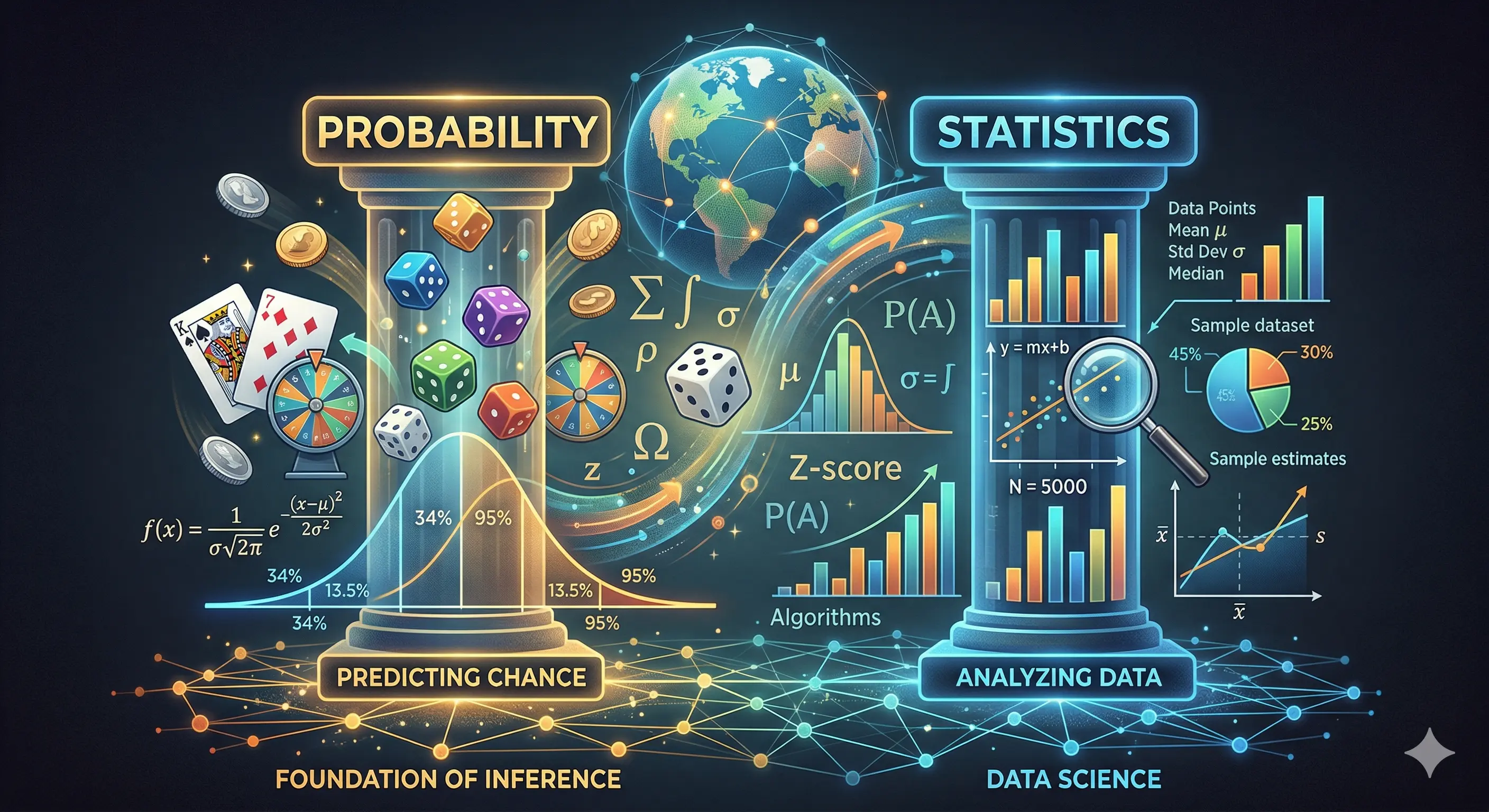
A common question for aspiring practitioners is how Machine Learning (ML) and
Artificial Intelligence intersect with the foundational pillars of Probability and Statistics.
While many experts emphasize that mastering these mathematical disciplines is
non-negotiable for data science excellence, the real challenge lies in pinpointing exactly
which concepts are essential for success in the field.
To demystify these connections, we are launching a five-part series designed to bridge
the gap between theory and application. Our goal is to move beyond dense technical
jargon and explain these core principles in clear, accessible terms, ensuring you build a
solid foundation for your journey into AI.
The Doctrine of Chance
In everyday language, we use “chance” to describe everything from a coin flip to a market
crash and every occurrence involves an element of uncertainty. While we often talk about
the chance of something happening, probability gives us the mathematical framework to
measure that uncertainty. By applying formal rules to these unknowns, we move beyond
guesswork - transforming raw outcomes into clear, actionable insights and a solid
foundation for decision making.
Formalizing the Unpredictability
We will now explore how to formally model uncertainty using a mathematical approach.
To get started, we must first define the core terminology.
- Random Experiment (R): An action with an uncertain outcome.
- Sample Space (Ω): The collection of all possible outcomes of R.
- Event (E): A specific subset of the sample space to which we assign probability.
To understand these concepts, we will use two classic examples namely “Toss a Coin”
and “Rolling a Die”.

| Random Experiment (R) | Sample Space (Ω) | Event (E) |
|---|---|---|
| Toss a Coin | {Head, Tail} | Head appears → {Head} |
| Rolling a Die | {1, 2, 3, 4, 5, 6} | A six appears → {6} |
Axioms of Probability
The three fundamental rules of Probability are -
- Non-Negativity: The probability of any event occurring must be a non-negative
real number. In a formal mathematical approach, this means that for any event 𝐴,
the probability 𝑃(𝐴) is always greater than or equal to zero. There is no such thing
as a negative chance of an event happening. Importantly, the probability of any
event is between zero and one.
$$ P(A) \in [0, 1] $$
- Certainty: The probability of the entire sample space is exactly 1. While every
individual prediction involves an element of uncertainty, the certainty that
something from the set of all possible outcomes will happen is absolute.
$$ P(\Omega) = 1 $$
- Additivity: If two events cannot happen at the same time (mutually exclusive), the
probability that either one or the other occurs is the sum of their individual
probabilities.
$$ P\left(\bigcup E_i\right) = \sum P(E_i) $$
Visualize the Relationship between Events
We can visually represent the four primary ways in which random events \(E_1\) and \(E_2\) interact within a probabilistic framework.
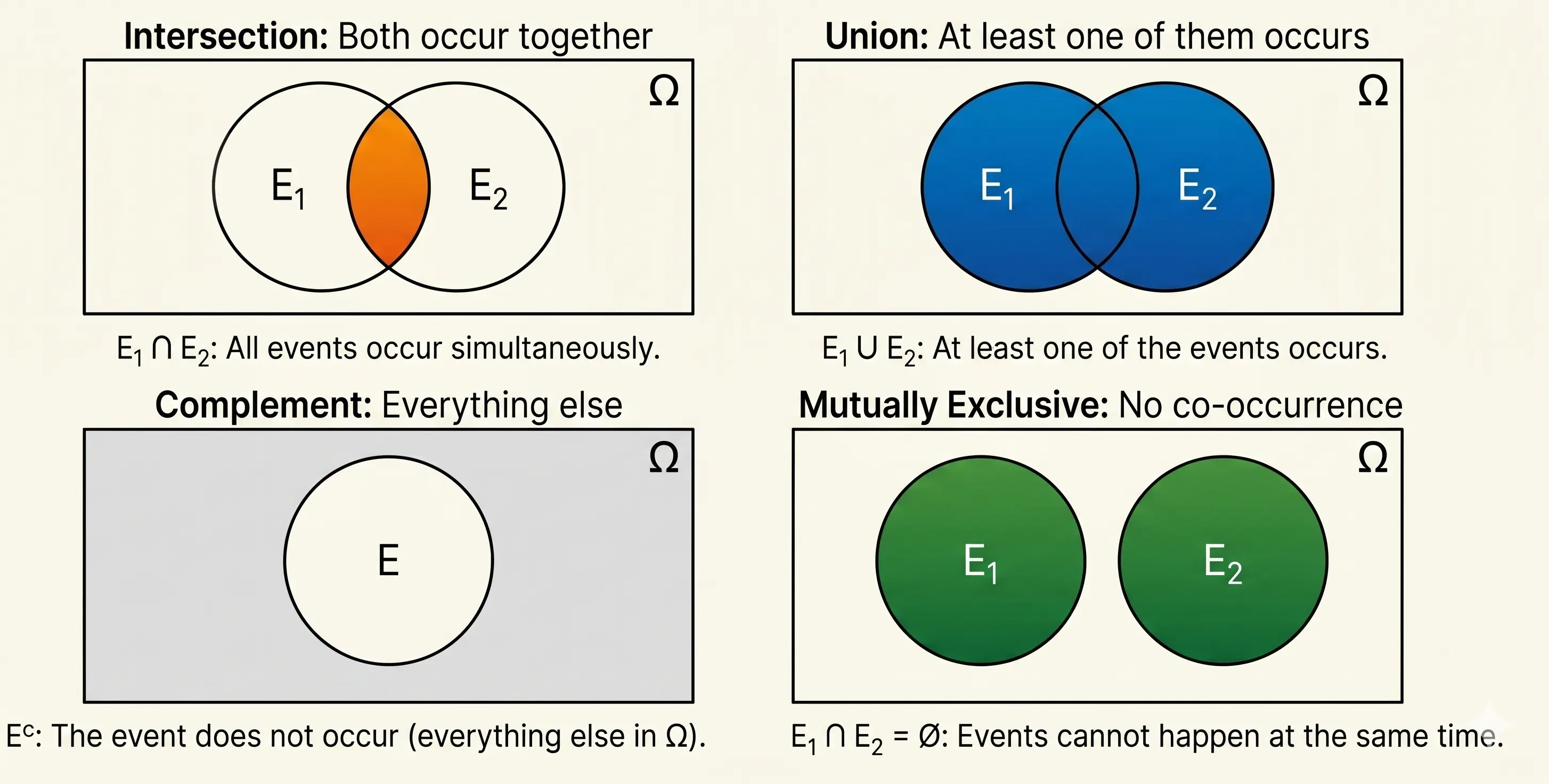
From the above logical relationship we can derive additional rules -
- For Complements: The probability of an event not happening is 1 minus the
probability that it does.
$$ P(A^c) = 1 - P(A) $$
- For Union: When adding the probabilities of two overlapping events, we
double-count their intersection. So, we need to subtract it once to get the
probability of true union.
$$ P(A \cup B) = P(A) + P(B) - P(A \cap B) $$
Conditional Probability and Independence
Conditional probability focuses on how the occurrence of one event (Event 𝐵) updates
our understanding of the probability of another (Event 𝐴). Conversely, it is the probability
of Event 𝐴 occurring under the assumption that Event 𝐵 is already confirmed or occurred.
The universe shrinks from Ω to 𝐵.
$$ P(A \mid B) = \frac{P(A \cap B)}{P(B)} $$
Two events A and B are independent if knowing B confirmed or occurred does not change
the probability of A.
$$ P(B \mid A) = \frac{P(B \cap A)}{P(A)} = \frac{P(A)P(B)}{P(A)} = P(B) $$
Note: If A and B are independent, their intersection is simply the product of their individual probabilities.
$$ P(A \cap B) = P(A)P(B) $$
The Law of Total Probability
For any event 𝐴, its probability can be determined by partitioning the sample space Ω
into smaller, manageable, disjoint and exhaustive scenarios \(B_i\) and summing up the conditional
probabilities of \(P(A \mid B_i)\) weighted by the likelihood of each subset \(P(B_i)\).
Here the entire sample space is divided into small, disjoint subsets \(B_i\).
Event \(A\) spans across multiple subsets.
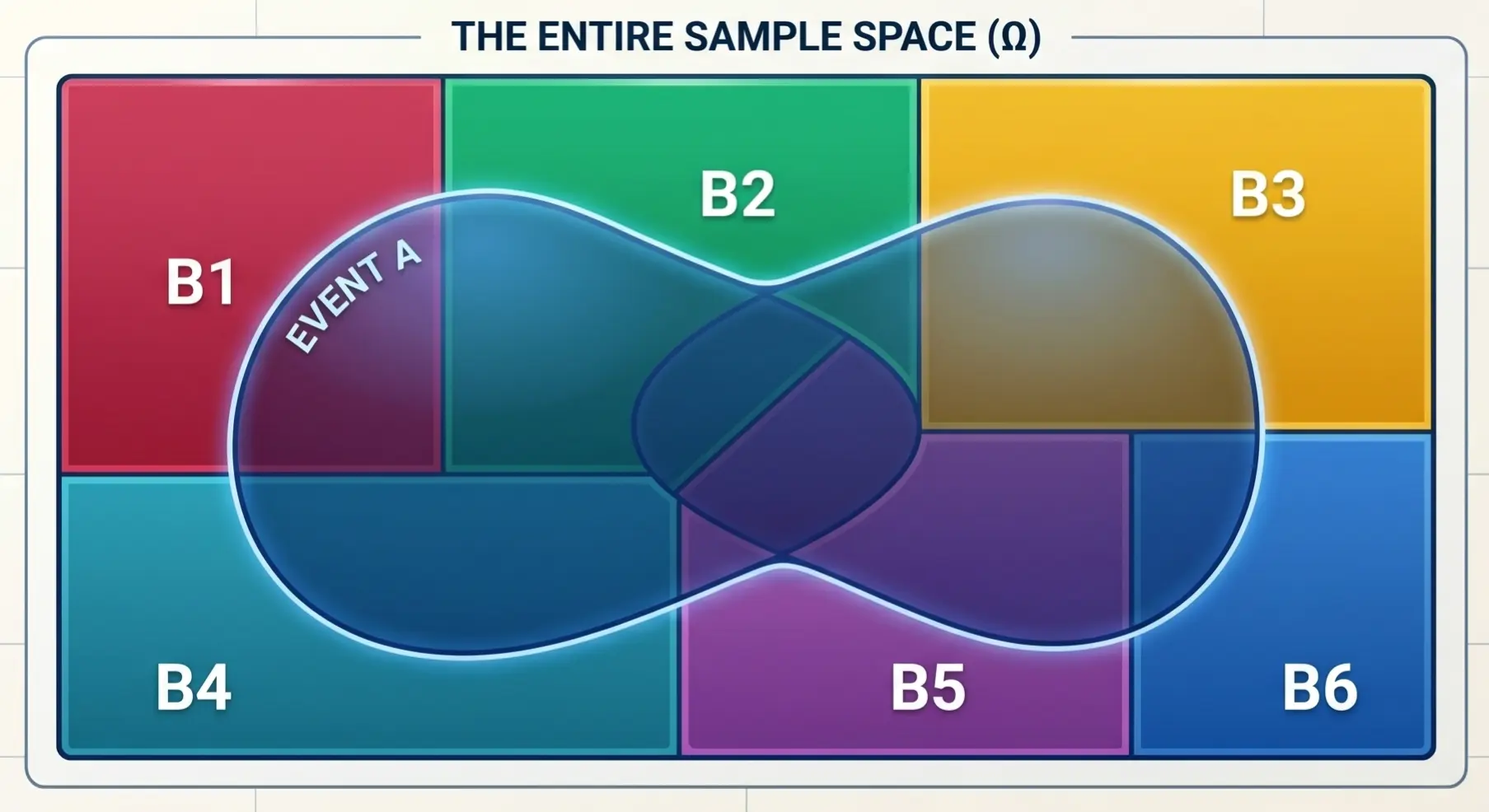
$$ P(A) = \sum_{i=1}^{n} P(A \mid B_i) \cdot P(B_i) $$
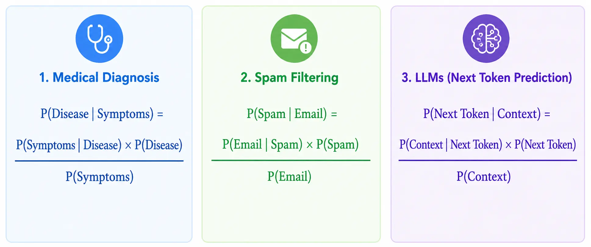
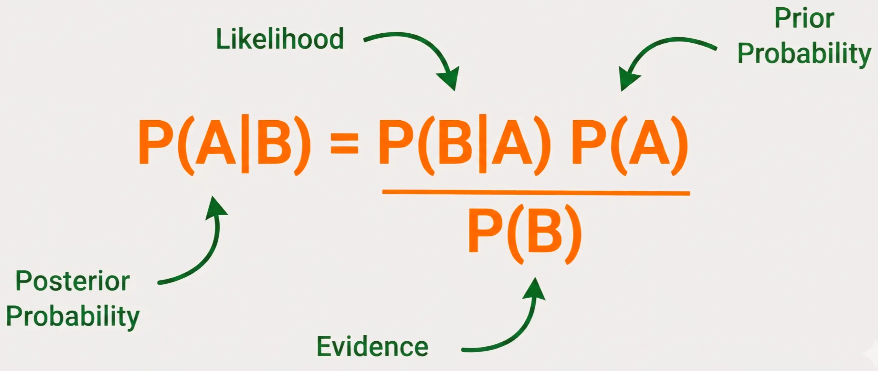
Bayes’ Theorem
It is a mathematical formula used to calculate the posterior probability (P(A|B)) (the
probability of event 𝐴 occurring given that event 𝐵 has already occurred). It uses the
likelihood (P(B|A)) to update the initial belief called prior probability of the event 𝐴 based on
new evidence (P(B)).
$$ P(A \mid B) = \frac{P(A \cap B)}{P(B)} \quad \text{assuming } P(B) > 0 $$
$$ P(A \mid B) = \frac{P(B \mid A) \cdot P(A)}{P(B)} \quad \text{because } P(B \mid A) = \frac{P(B \cap A)}{P(A)} $$
$$ P(A \mid B) = \frac{P(B \mid A) \cdot P(A)} {\sum_{i=1}^{n} P(B \mid A_i) \cdot P(A_i)} \quad \text{by applying the law of total probability} $$
For any event \(A_j\) from the sample space of A -
$$ P(A_j \mid B) = \frac{P(B \mid A_j) \cdot P(A_j)} {\sum_{i=1}^{n} P(B \mid A_i) \cdot P(A_i)} \quad \text{} $$
At its core, Bayes’ Theorem is a mathematical framework for learning. It provides a rigorous way to update our beliefs, predictions, or diagnoses when we are presented with new evidence. Instead of treating probability as a fixed, one-time calculation, Bayes’ Theorem treats it as a dynamic process: we start with an initial assumption, apply new data, and arrive at a more accurate conclusion. Because it excels at handling uncertainty, it is the invisible engine powering many of the systems we rely on a daily basis.
For instance, Bayes’ Theorem helps diagnose medical conditions by weighing a patient’s test results against the actual prevalence of the disease in the broader population. It also powers email spam filters, which analyze massive volumes of messages to establish a baseline probability of an email being junk. In the realm of artificial intelligence, Large Language Models depend heavily on this same Bayesian logic. When an application predicts the next word you will type, it is solving a conditional probability problem. The algorithm uses your previously typed words as context to determine the likelihood of the subsequent word. Each new word you enter provides fresh evidence, instantly narrowing down the universe of possibilities.