In the first part we have seen how to represent the uncertainty around events and attach numerical values to quantify their likelihood mathematically which is called Probability. In this article, we are going to deep dive into the realm of Random Variables by navigating through the abstraction of physical events.
Demystifying Random Variables
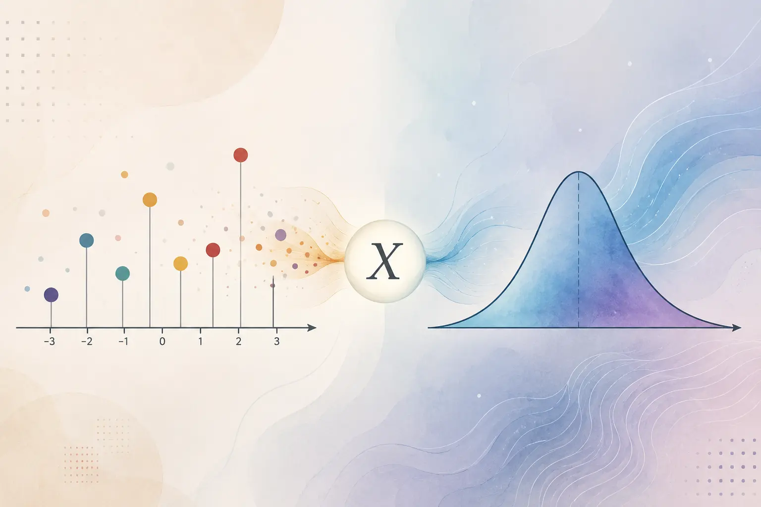
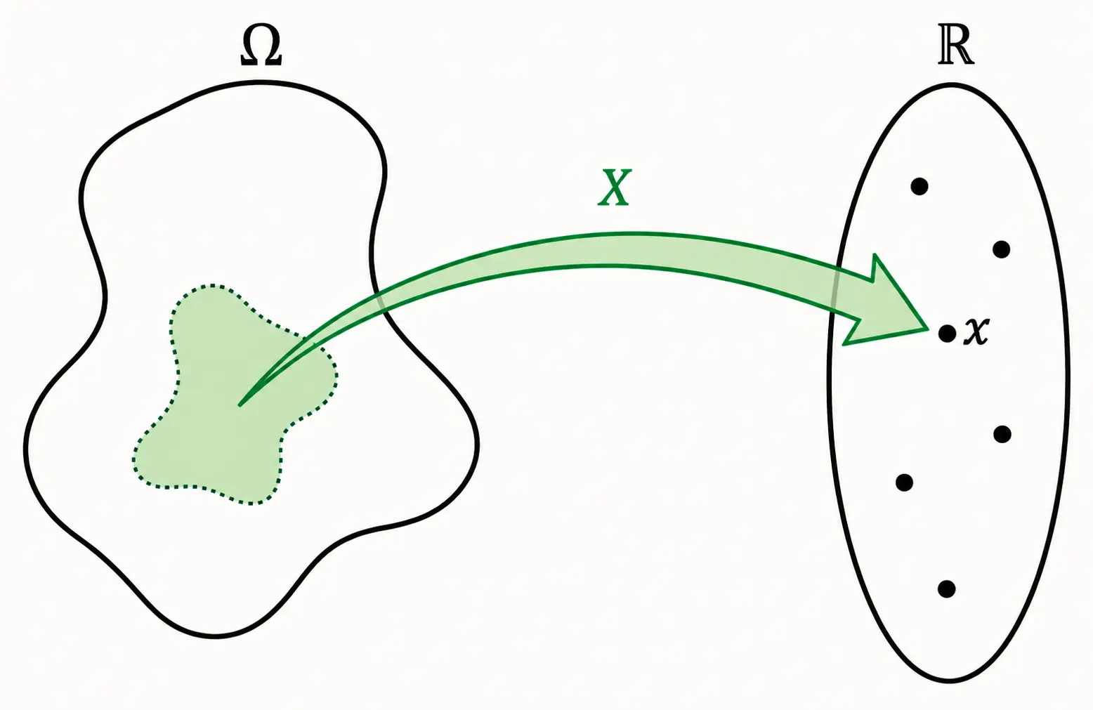
An event or any physical event is a qualitative term like Head/Tail, value of the face of a rolled dice etc. A random variable is a function that translates these qualitative outcomes from sample space Ω into measurable numerical values which is a real number ℝ. The advantage of this mapping to a real number is to enable the computation using Statistics, Calculus and Algebra.
$$ \text{Random Variable } X:\Omega \rightarrow \mathbb{R} $$
If two fair dice are rolled then, Sample Space Ω contains 36 pairs {(1, 1), (1, 2), ….., (5, 6), (6, 6)}. If we consider that random variable \(X\) represents the sum of faces, then an event that sum of faces is 3 can be represented numerically ℝ by following observations {(1, 2), (2, 1)} that contribute to the event because their sum is 3; thus \(X\) maps the events {(1, 2), (2, 1)} to the number 3.
There are 2 pairs, namely {(1,2), (2,1)}, whose sum equals 3.
Since the sample space contains 36 equally likely outcomes,
$$ P(X=3)=\frac{2}{36} $$
Any specific value of random variable \(X\) is specified by lowercase \(x\). The significance of random variables lies in the fact that random variables are the mathematical foundation of AI and ML. In any AI/ML use case, algorithms rely on random variables that represent the attributes of the observations allowing algorithms to identify atterns, learn and make decisions.
The Great Divide
A random variable (RV) can take different values - it can be Discrete or Continuous and basis that it can either be discrete RV or continuous RV. There are different mathematical approaches to deal with them separately.
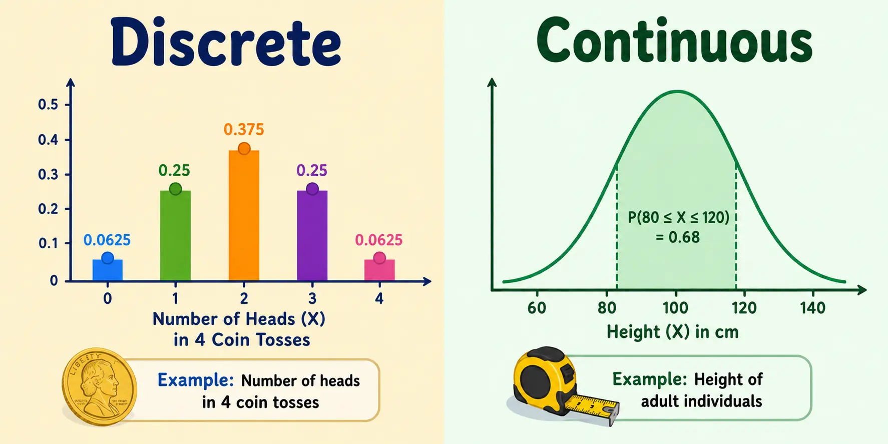
- Discrete RV: It takes finite or countably infinite values. Example: Number of calls to an office in a certain duration, If an email is spam/valid, Number of heads in 4 coin tosses etc.
- Continuous RV: It takes any value in an uninterrupted range; basically uncountable and infinite possible values in a range. Example: Weight of humans, Time to complete a 100 meter race, Height of adult individuals etc.
The Mathematical Engine
We need to understand how to deal with different forms of random variables separately. To achieve this mathematically we need to master a few basic concepts that drive probability calculations of discrete and continuous random variables.
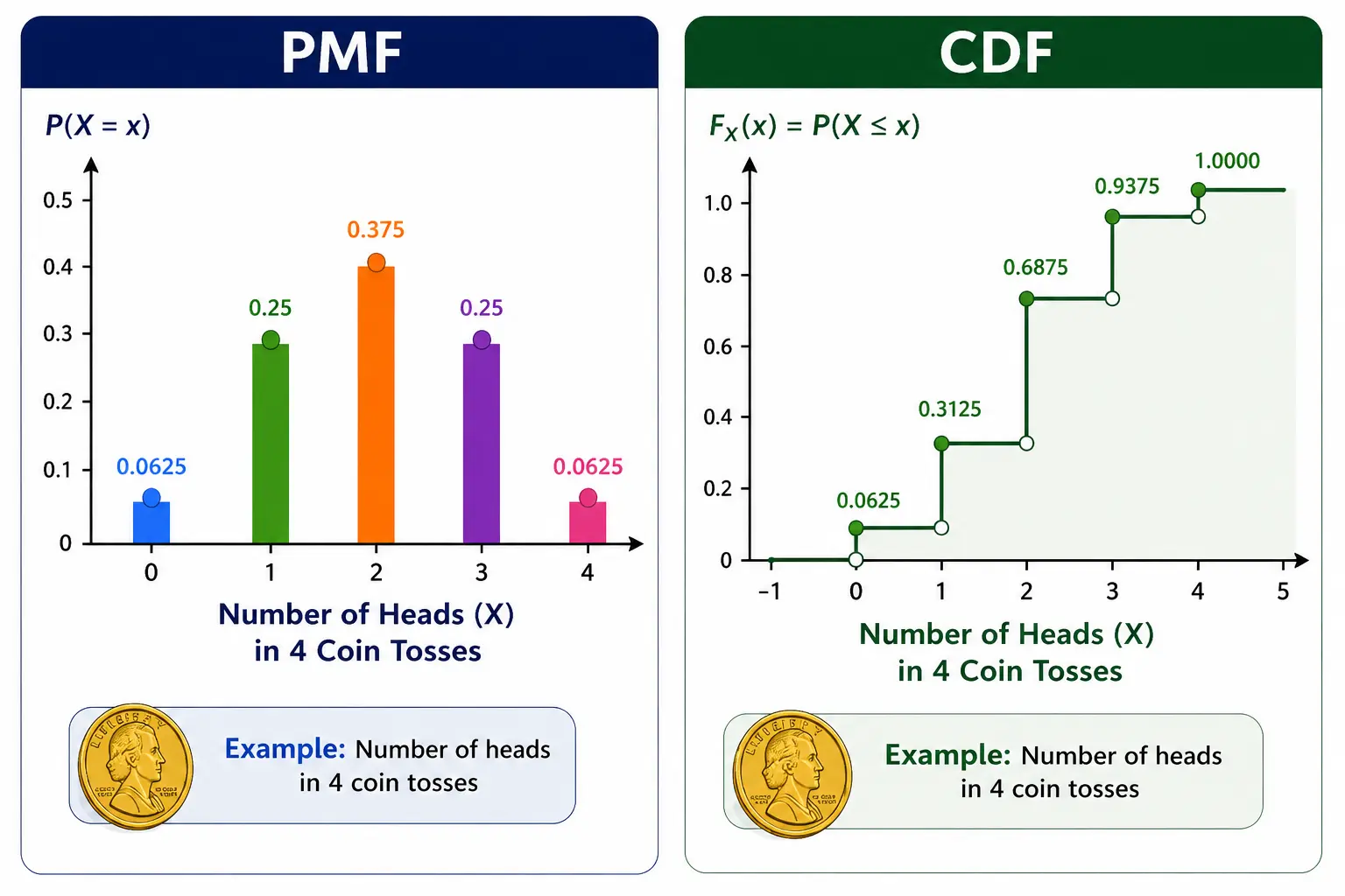
Probability Mass Function (PMF): It is the probability accumulated at specific values \(x\) that a Discrete RV \(X\) takes (P(X=x)). It adheres to all the axioms of probability.
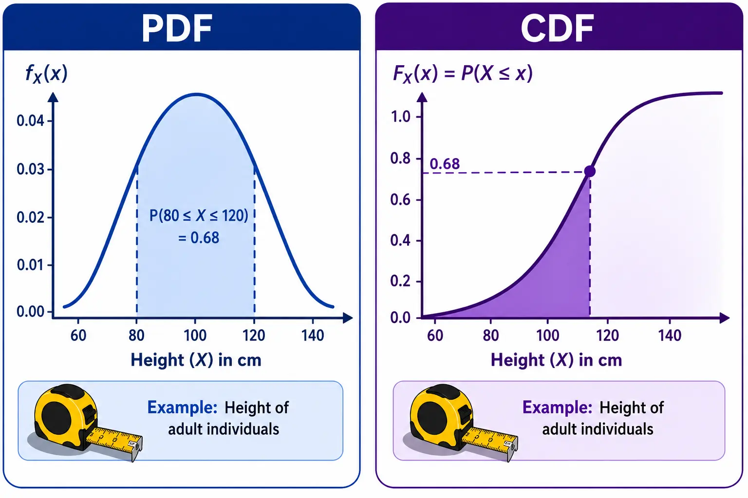
Cumulative Distribution Function (CDF): It is the actual probability (running total) that a RV will be less or equal to a particular value \(F_X(x) = P(X \le x)\). CDF is applicable to both discrete and continuous random variables. Since it is a probability, it also follows the axioms, starts at 0, non-decreasing, right continuous and ends at 1. The probability that \(P(X \le 3)\) is calculated as below.
$$ \begin{align} P(X \le 3) &= P(X \le 0)+P(X \le 1)+P(X \le 2)+P(X \le 3) \ \end{align} $$ $$ \begin{align} P(X \le 3) &= 0+0.0625+0.25+0.375+0.25 \ \end{align} $$ $$ \begin{align} P(X \le 3) &= 0.9375 \end{align} $$
The cumulative probability at different values is then plotted to derive the CDF plot.
- Probability Distribution Function (PDF): It is used to calculate the probability for a Continuous RV. It also adheres to all the axioms of probability. Since the probability at any single point for a continuous RV is 0 \(P(X=x)=0\), PDF is measured as the area under the curve over an interval \(P(a \le X \le b) = \int_{a}^{b} f(x)dx\). The CDF of continuous RV is calculated as \(F(a) = \int_{-\infty}^{a} f(x)dx\). For continuous RVs, the derivative of CDF is PDF and integration of PDF over an interval is the CDF.
Describing a Random Variable
When we try to describe a random variable and derive its attributes, we do it through the form or distribution it takes. The distribution of a random variable refers to how the different values of that variable are spread out across observations; basically the shape if inspected visually of the random variable. We will discuss the following important properties of a random variable.
- Mean/Expectation: It is the probability-weighted average of all the possible values of the random variable.
$$ E(X)=\sum_x x\cdot P(X=x) \qquad \text{for discrete RV} $$
$$ E(X)=\int_{-\infty}^{\infty} x\cdot f(x)dx \qquad \text{for continuous RV} $$
- Variance: The spread of the values of the random variable from mean.
$$ Var(X)=E[(X-E(X))^2] $$
$$ Var(X)=E[X^2-2XE(X)+E(X)^2] $$
$$ Var(X)=E(X^2)-2E(X)E(X)+E(X)^2 $$
$$ Var(X)=E(X^2)-E(X)^2 $$
$$ Var(aX)=a^2Var(X) $$
- Standard Deviation: The unit-of-measure (UoM) of variance is square of the original UoM of the random variable. Standard deviation is the square root of the variance that measures the spread in the original UoM.
$$ Std.Dev(X)=\sqrt{Var(X)} $$
- Mode: Mode is the most frequent value that appears in the set of values that the RV takes.
$$ \text{Dataset: } {1,2,2,3,4}; \quad \text{Mode} = 2 $$
- Median: If the values of a RV are sorted either from lowest to highest or highest to lowest then the middle value that splits the data exactly in half is called the Median.
$$ \text{Dataset: } {3,1,7,9,5}; \quad \text{Median} = 5 $$
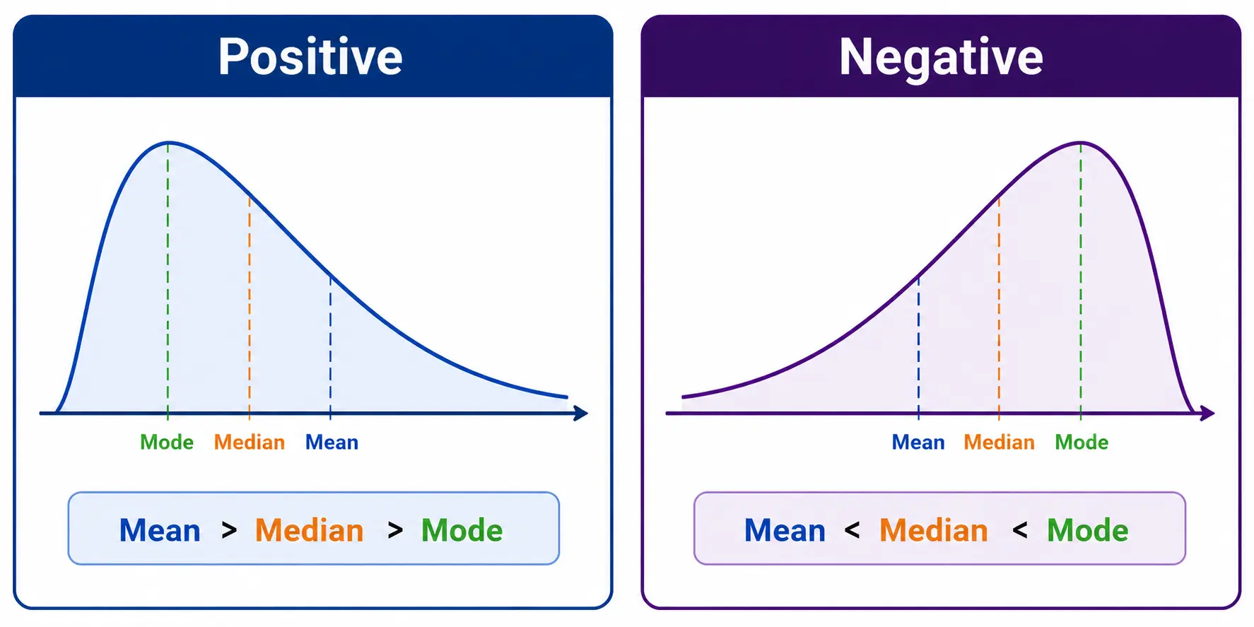
- Skewness: It measures the asymmetry of a distribution i.e. if the values are evenly spread from mean or leaned towards one side.
Properties of Mean
These are the elementary properties of mean/expectation.
If \(X \ge 0\), then \(E(X) \ge 0\).
If \(a \le X \le b\), then \(a \le E(X) \le b\).
If \(c\) is constant then \(E(c) = c\).
For a function of \(X\) -
$$ \text{Let}, Y = g(X) $$
$$ E(Y) = E(g(X)) $$
$$ E(Y) = \sum_x g(X = x) \cdot P(X = x) $$
- Linearity of expectation -
$$ E(aX+b) = a \cdot E(X) + E(b) = aE(X) + b $$
- Similar to Law of Total Probability, Total Expectation Theorem can also be defined as below.
$$ E(X)=P(A_1)E(X\mid A_1)+P(A_2)E(X\mid A_2)+\cdots+P(A_n)E(X\mid A_n) $$
Common Random Variables
We now focus on a few common random variables, their usage, key properties and shape of the distribution.
Discrete Random Variables
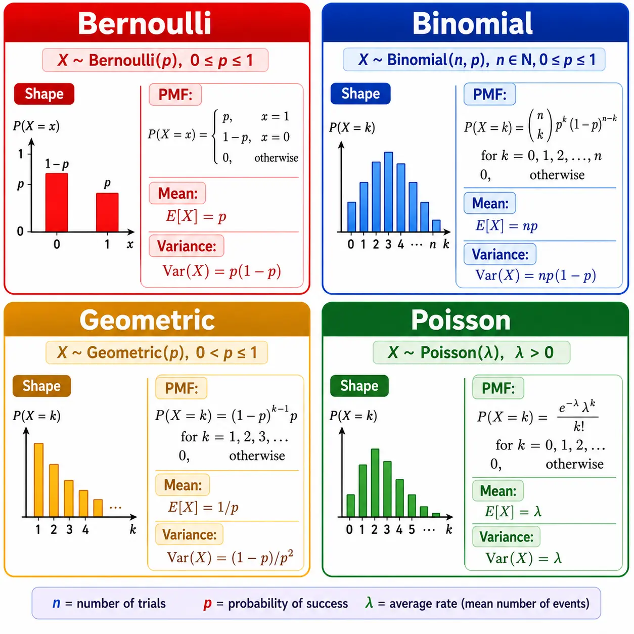
Bernoulli Distribution: It can be thought of a model for the experiment whose outcome is binary i.e. head/tail, yes/no etc. The outcome is positive with probability \(p\) and negative with probability \(1-p\).
Binomial Distribution: This distribution with parameter \(n\) and \(p\) is the generalized case of Bernoulli distribution where \(n\) is the number of sequences of independent random experiments or trials and \(p\) is the probability of a positive outcome in each experiment. We can think of it as experiments like tossing a coin 20 times and calculating the probability of getting 9 heads where the probability of head in each trial is 0.6.
Geometric Distribution: This type of distribution is to model the number of Bernoulli trials with probability \(p\) of success until first success like throwing a die multiple times until ‘1’ appears for the first time.
Poisson Distribution: This distribution is to model the probability of a given number of events \(k\) occurring in a fixed interval of time or space if these events occur with a known constant mean rate \(\lambda (> 0)\). and independently of the time since the last event. The examples include the number of phone calls received by a call center or the number of emails per day etc.
Continuous Random Variables
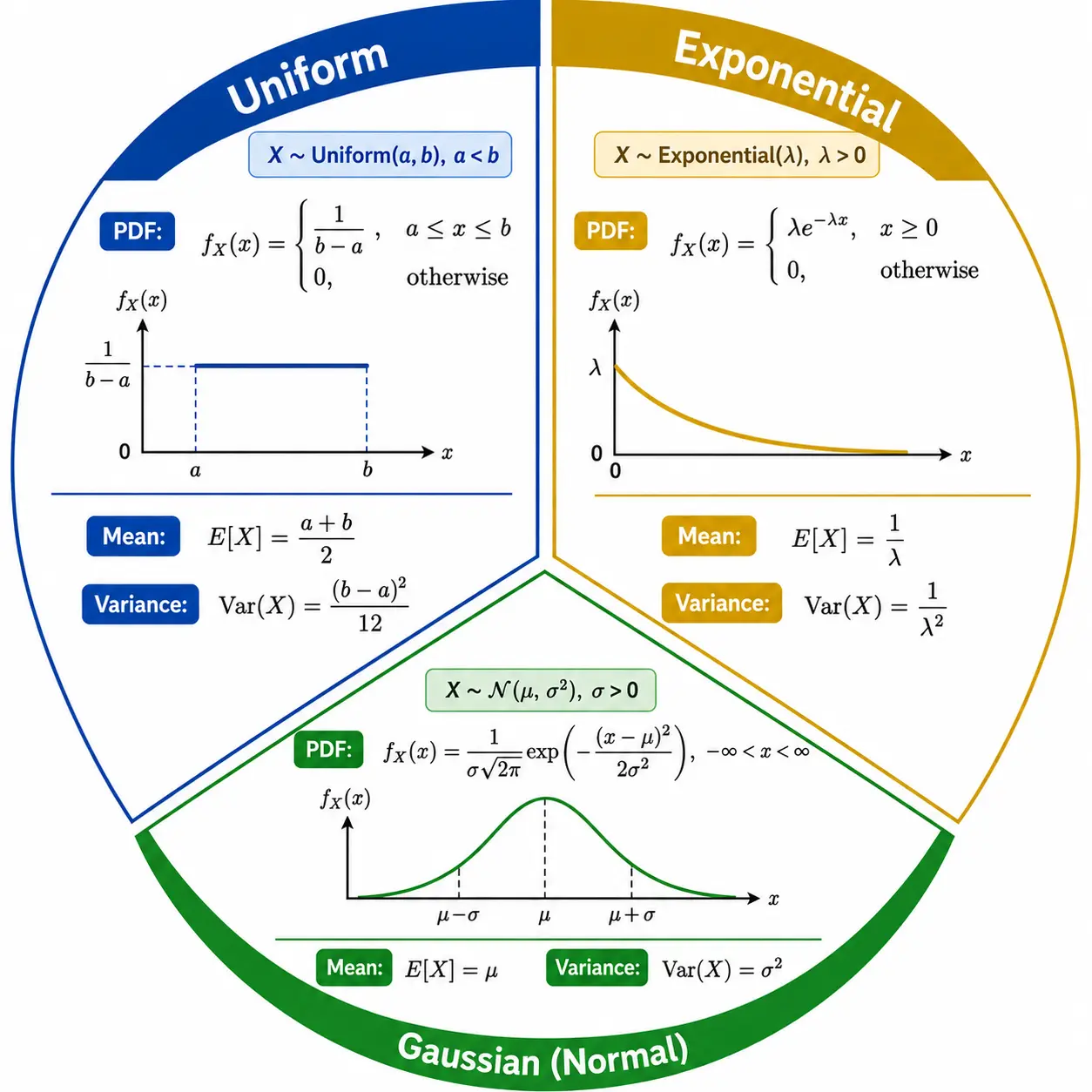
Uniform Distribution: It describes an experiment where the outcome is continuous and it can take any value between a minimum and maximum value denoted as \(a\) and \(b\). One of the examples can be a random number generator.
Exponential Distribution: It is used to model the probability distribution of the time between processes in which events occur continuously and independently at a constant average rate \(\lambda (> 0)\) like the amount of time from now until an electric bulb failure (the of the bulb). One of the important properties of Exponential distribution is Memorylessness which can be explained as the probability of an event happening in the future is completely unaffected by how much time has already passed. For example, the probability of waiting 10 more minutes is the same regardless of whether you just arrived or have been waiting for hours; the system has no memory of how long it has already been waiting.
Gaussian Distribution: This distribution is used to represent any real valued random variable whose distribution is unknown. Mean \(\mu\) and Variance \(\sigma^2\) are used to denote it. If we plot the number of words for each tweet in a set of tweets we can see the shape follows a Bell Curve which is symmetric where most of the data points are centered around the mean and conclude that the distribution is Gaussian or Normal. This distribution is very important and forms the foundation for much of statistical inference.